pdf("pp.pdf",width=8,height=8)
#pdf("pp.pdf",width=8,height=8)
par(mar=c(3.5,2.5,3,1))
par(mgp=c(1.5,0.3,0))
par(tck=-0.02)
par(mfrow = c(3, 5))
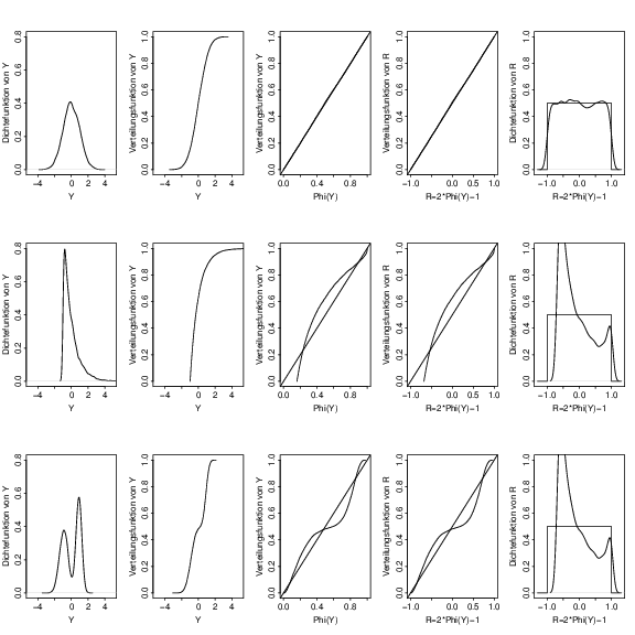
h <- (seq(1, 10000) - 0.5)/10000
x1 <- rnorm(10000)
plot(density(x1), type = "l", lty = 1, main="", xlab = "Y", ylab =
"Dichtefunktion von Y", xlim = c(-5, 5), ylim = c(0, 0.8))
plot(sort(x1), h, type = "l", lty = 1, xlab = "Y", ylab =
"Verteilungsfunktion von Y", main="", xlim = c(-5, 5), ylim = c(0, 1))
plot(sort(pnorm(scale(x1))), h, type = "l", lty = 1, main="", xlab = "Phi(Y)",
ylab = "Verteilungsfunktion von Y", xlim = c(0, 1), ylim = c(0,
1))
abline(0, 1)
plot(2 * sort(pnorm(scale(x1))) - 1, h, type = "l", lty = 1, main="", xlab =
"R=2*Phi(Y)-1", ylab = "Verteilungsfunktion von R", xlim = c(-1,
1), ylim = c(0, 1))
abline(0.5, 0.5)
plot(density(2 * sort(pnorm(scale(x1))) - 1, width = 0.3), type = "l",
lty = 1, xlab = "R=2*Phi(Y)-1", ylab = "Dichtefunktion von R",
main="", xlim = c(-1.3, 1.3), ylim = c(0, 1))
lines(x = c(-1.3, -1, -1, 1, 1, 1.3), y = c(0, 0, 0.5, 0.5, 0, 0))
x2 <- scale(rchisq(10000, 2))
plot(density(x2), type = "l", lty = 1, main="", xlab = "Y", ylab =
"Dichtefunktion von Y", xlim = c(-5, 5), ylim = c(0, 0.8))
plot(sort(x2), h, type = "l", lty = 1, main="", xlab = "Y", ylab =
"Verteilungsfunktion von Y", xlim = c(-5, 5), ylim = c(0, 1))
plot(sort(pnorm(scale(x2))), h, type = "l", lty = 1, main="", xlab = "Phi(Y)",
ylab = "Verteilungsfunktion von Y", xlim = c(0, 1), ylim = c(0,
1))
abline(0, 1)
plot(2 * sort(pnorm(scale(x2))) - 1, h, type = "l", lty = 1, main="", xlab =
"R=2*Phi(Y)-1", ylab = "Verteilungsfunktion von R", xlim = c(-1,
1), ylim = c(0, 1))
abline(0.5, 0.5)
plot(density(2 * sort(pnorm(scale(x2))) - 1, width = 0.3), main="", type = "l",
lty = 1, xlab = "R=2*Phi(Y)-1", ylab = "Dichtefunktion von R",
xlim = c(-1.3, 1.3), ylim = c(0, 1))
lines(x = c(-1.3, -1, -1, 1, 1, 1.3), y = c(0, 0, 0.5, 0.5, 0, 0))
x3 <- scale(c(rnorm(5000, -2, 1), rnorm(5000, 1.5, 0.6)))
plot(density(x3), type = "l", lty = 1, main="", xlab = "Y", ylab =
"Dichtefunktion von Y", xlim = c(-5, 5), ylim = c(0, 0.8))
plot(sort(x3), h, type = "l", lty = 1, main="", xlab = "Y", ylab =
"Verteilungsfunktion von Y", xlim = c(-5, 5), ylim = c(0, 1))
plot(sort(pnorm(scale(x3))), h, type = "l", lty = 1, main="", xlab = "Phi(Y)",
ylab = "Verteilungsfunktion von Y", xlim = c(0, 1), ylim = c(0,
1))
abline(0, 1)
plot(2 * sort(pnorm(scale(x3))) - 1, h, type = "l", lty = 1, main="", xlab =
"R=2*Phi(Y)-1", ylab = "Verteilungsfunktion von R", xlim = c(-1,
1), ylim = c(0, 1))
abline(0.5, 0.5)
plot(density(2 * sort(pnorm(scale(x2))) - 1, width = 0.3), type = "l",
lty = 1, xlab = "R=2*Phi(Y)-1", ylab = "Dichtefunktion von R",
main="", xlim = c(-1.3, 1.3), ylim = c(0, 1))
lines(x = c(-1.3, -1, -1, 1, 1, 1.3), y = c(0, 0, 0.5, 0.5, 0, 0))
dev.off()
library(classPP)
# 1-dim Projection
data(iris)
ir <- scale(iris[,1:4])
# auf PC1
library(MVA)
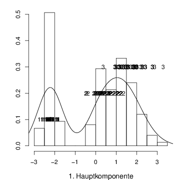
a <- princomp(ir)
pdf("pproj0.pdf",width=5,height=5)
par(mar=c(4,4,1,1))
hist(a$sco[,1],freq=F,
xlab="1. Hauptkomponente",ylab="",main="",cex.lab=1.2)
lines(density(a$sco[,1]))
grp<-c(rep(1,50),rep(2,50),rep(3,50))
text(a$sco[,1],grp/10,grp)
dev.off()
library(classPP)
# 1-dim Projection
data(iris)
ir <- scale(iris[,1:4])
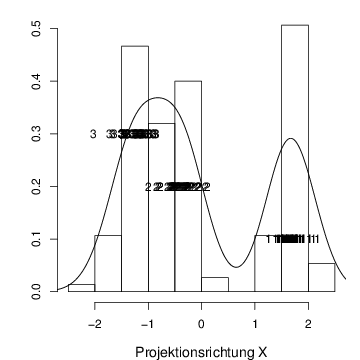
PP.opt<-PP.optimize.Huber("LDA",1,ir,iris[,5],cooling=0.999,r=1)
pdf("pproj1.pdf",width=5,height=5)
par(mar=c(4,4,1,1))
hist(as.matrix(ir)%*%PP.opt$proj.best,freq=F,
xlab="Projektionsrichtung X",ylab="",main="",cex.lab=1.2)
lines(density(as.matrix(ir)%*%PP.opt$proj.best))
grp<-c(rep(1,50),rep(2,50),rep(3,50))
text(as.matrix(ir)%*%PP.opt$proj.best,grp/10,grp)
dev.off()
library(classPP)
# 1-dim Projection
data(iris)
ir <- scale(iris[,1:4])
# 2d-Dichteschaetzung:
set.seed(101)
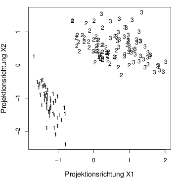
PP.opt<-PP.optimize.Huber("LDA",2,ir,iris[,5],cooling=0.999,r=1)
pdf("pproj2.pdf",width=5,height=5)
par(mar=c(4,4,1,1))
plot(as.matrix(ir)%*%PP.opt$proj.best,type="n",
xlab="Projektionsrichtung X1",ylab="Projektionsrichtung X2",main="",cex.lab=1.2)
text(as.matrix(ir)%*%PP.opt$proj.best,label=grp)
dev.off()
library(classPP)
# 1-dim Projection
data(iris)
ir <- scale(iris[,1:4])
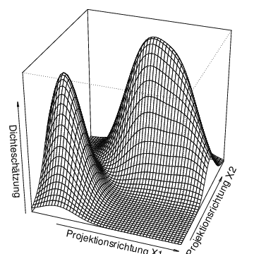
# 2d-Dichteschaetzung:
library(MASS)
projdat <- as.matrix(ir)%*%PP.opt$proj.best
f2 <- kde2d(projdat[,1], projdat[,2], n = 50)
pdf("pproj3.pdf",width=5,height=5)
par(mar=c(0,0,0,0))
persp(f2, phi = 30, theta = 20, d = 5,
xlab="Projektionsrichtung X1",ylab="Projektionsrichtung X2",
zlab="Dichteschätzung",cex.lab=1.2)
dev.off()