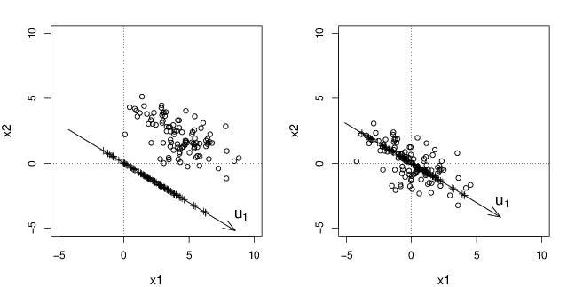
# Figure for mean-centering PCs
pdf("pcamean.pdf",width=9,height=4.5)
par(mfrow=c(1,2))
par(mar=c(4,4,2,2))
library(mvtnorm)
set.seed(300)
x=rmvnorm(100,c(4,2),matrix(c(4,-1.9,-1.9,2),ncol=2))
plot(x,xlim=c(-5,10),ylim=c(-5,10),xlab="x1",ylab="x2",cex.lab=1.2)
e=eigen(cov(x))
l1=-e$vectors[,1]
l12=-e$vectors[,1:2]
s1=x%*%l1
c1=5;c2=10;arrows(-l1[1]*c1,-l1[2]*c1,l1[1]*c2,l1[2]*c2,length=0.20,angle=20)
t1=cbind(s1,rep(0,nrow(x)))
t1rot=t1%*%t(l12)
points(t1rot,pch=3)
abline(h=0,lty=3)
abline(v=0,lty=3)
text(9,-4,expression(u[1]),cex=1.4)
x.mc=scale(x,T,F)
plot(x.mc,xlim=c(-5,10),ylim=c(-5,10),xlab="x1",ylab="x2",cex.lab=1.2)
s1=x.mc%*%l1
c1=6;c2=8;arrows(-l1[1]*c1,-l1[2]*c1,l1[1]*c2,l1[2]*c2,length=0.20,angle=20)
t1=cbind(s1,rep(0,nrow(x)))
t1rot=t1%*%t(l12)
points(t1rot,pch=3)
abline(h=0,lty=3)
abline(v=0,lty=3)
text(7,-3,expression(u[1]),cex=1.4)
dev.off()
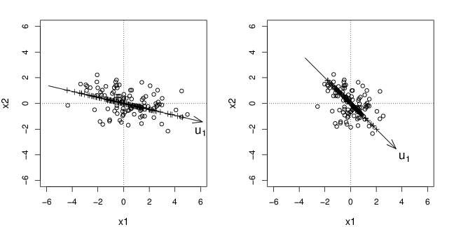
# Figure for scaling PCs
pdf("pcascale.pdf",width=9,height=4.5)
par(mfrow=c(1,2))
par(mar=c(4,4,2,2))
library(mvtnorm)
set.seed(300)
x=rmvnorm(100,c(0,0),matrix(c(4,-0.9,-0.9,1),ncol=2))
plot(x,xlim=c(-6,6),ylim=c(-6,6),xlab="x1",ylab="x2",cex.lab=1.2)
x.pc=princomp(x)
l1=-x.pc$loa[,1]
l12=x.pc$loa[,1:2]
s1=x.pc$sco[,1]
c1=6;c2=6.3;arrows(-l1[1]*c1,-l1[2]*c1,l1[1]*c2,l1[2]*c2,length=0.20,angle=20)
t1=cbind(s1,rep(0,nrow(x)))
t1rot=t1%*%t(l12)
points(t1rot,pch=3)
abline(h=0,lty=3)
abline(v=0,lty=3)
text(6,-2.2,expression(u[1]),cex=1.4)
x.sc=scale(x,T,T)
plot(x.sc,xlim=c(-6,6),ylim=c(-6,6),xlab="x1",ylab="x2",cex.lab=1.2)
x.pc=princomp(x.sc)
l1=-x.pc$loa[,1]
l12=x.pc$loa[,1:2]
s1=x.pc$sco[,1]
c1=5;c2=5;arrows(-l1[1]*c1,-l1[2]*c1,l1[1]*c2,l1[2]*c2,length=0.20,angle=20)
t1=cbind(s1,rep(0,nrow(x)))
t1rot=t1%*%t(l12)
points(t1rot,pch=3)
abline(h=0,lty=3)
abline(v=0,lty=3)
text(4.2,-4.2,expression(u[1]),cex=1.4)
dev.off()