2.8 Quantile-Quantile Plots

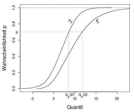
		# Quantile Quantile Plots pdf("quanquan.pdf",width=6,height=5) par(mar=c(4.5,4.5,1,1)) set.seed(100) n <- 10000 # Normalverteilung xn <- rnorm(n,7,3) xp <- (seq(1,n)-0.5)/n xns <- sort(xn) plot(xns,xp,type="l",xlim=c(-2,22), xlab="Quantil",ylab="Wahrscheinlichkeit p",cex.lab=1.3) # chi2-Verteilung xc <- rchisq(n,10) xcs <- sort(xc) lines(xcs,xp) abline(1,0,lty=2) sel <- 7000 segments(-10,xp[sel],xcs[sel],xp[sel],lty=3,cex=1.2) segments(xns[sel],-1,xns[sel],xp[sel],lty=3,cex=1.2) segments(xcs[sel],-1,xcs[sel],xp[sel],lty=3,cex=1.2) mtext("q (p)",side=1,at=8.8) mtext("y",side=1,at=8.5,line=0.5) mtext("q (p)",side=1,at=12) mtext("x",side=1,at=11.7,line=0.5) par(las=1) mtext("p",side=2,at=0.7,line=0.5) text(8.8,0.84,"F") text(9.2,0.82,"y") text(15.3,0.84,"F") text(15.5,0.82,"x") dev.off()
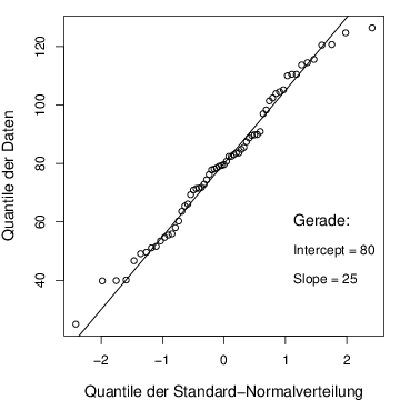
		# Quantile Quantile Plots # Buffalo Snowfall Daten data(buffalo,package="gss") dat <- buffalo pdf("qqnorma.pdf",width=5,height=5) par(mar=c(4,4,1,1)) qqnorm(dat,main="",xlab="Quantile der Standard-Normalverteilung", ylab="Quantile der Daten",cex.lab=1.2) abline(80,25) text(1,60,"Gerade:",cex=1.2,pos=4) text(1,50,"Intercept = 80",pos=4) text(1,40,"Slope = 25",pos=4) segments(0,0,0,3.6,lty=3) segments(1,0,1,3.6+0.75,lty=3) segments(-4,3.6,0,3.6,lty=3) segments(-4,3.6+0.75,1,3.6+0.75,lty=3) dev.off()
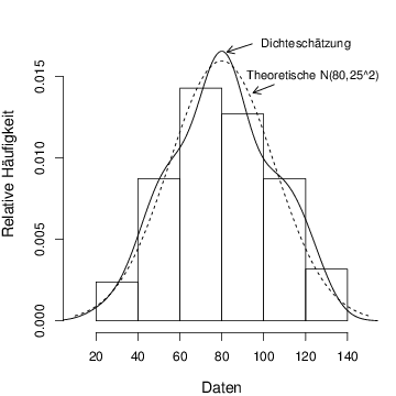
		# Quantile Quantile Plots # Buffalo Snowfall Daten data(buffalo,package="gss") dat <- buffalo pdf("qqnormb.pdf",width=5,height=5) par(mar=c(4,4,1,1)) hist(dat,freq=F,main="",ylim=c(0,0.018),xlim=c(10,150), xlab="Daten",ylab="Relative Häufigkeit",cex.lab=1.2) lines(density(dat)) lines(seq(10,150),dnorm(seq(10,150),80,25),lty=2) text(88,0.015,"Theoretische N(80,25^2)",pos=4,cex=0.9) arrows(105,0.0145,95,0.014,0.1) text(95,0.017,"Dichteschätzung",pos=4,cex=0.9) arrows(94.5,0.017,82.5,0.0165,0.1) dev.off()