# Normally distributed data
pdf("cdf1.pdf",width=5,height=5)
par(mar=c(4,4,1,1))
set.seed(101)
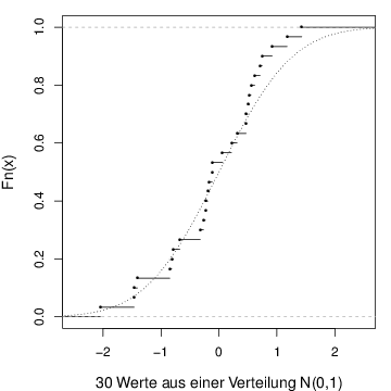
plot(ecdf(rnorm(30)),xlim=c(-2.5,2.5),pch=16,cex=0.5,main="",cex.lab=1.2,
xlab="30 Werte aus einer Verteilung N(0,1)")
a <- seq(-4,4,0.01)
lines(a,pnorm(a),lty=3)
dev.off()
# Normally distributed data
pdf("cdf2.pdf",width=5,height=5)
par(mar=c(4,4,1,1))
set.seed(101)
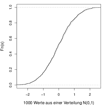
plot(ecdf(rnorm(1000)),xlim=c(-2.5,2.5),main="",cex.lab=1.2,
xlab="1000 Werte aus einer Verteilung N(0,1)")
a <- seq(-4,4,0.01)
lines(a,pnorm(a),lty=3)
dev.off()
# Kola Daten
data(chorizon,package="StatDA")
dat <- chorizon$Sc_INAA
pdf("cdf3.pdf",width=5,height=5)
par(mar=c(4,4,1,1))
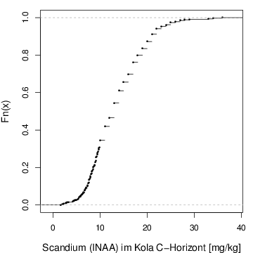
plot(ecdf(dat),pch=16,cex=0.5,main="",cex.lab=1.2,
xlab="Scandium (INAA) im Kola C-Horizont [mg/kg]")
dev.off()
# Kola Daten
data(ohorizon,package="StatDA")
dat <- ohorizon$Ni
pdf("cdf4.pdf",width=5,height=5)
par(mar=c(4,4,1,1))
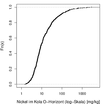
plot(ecdf(log10(dat)),pch=16,cex=0.5,main="",cex.lab=1.2,xaxt="n",
xlab="Nickel im Kola O-Horizont (log-Skala) [mg/kg]")
axis(1,at=log10(alog<-sort(c((10^(-50:50))%*%t(10)))),labels=alog)
dev.off()