set.seed(123)
x <- rnorm(100)
xout <- c(x,20)
pdf("scottfd1.pdf",width=8,height=5)
par(mfrow=c(2,2))
par(mar=c(4.5,4.5,1,1))
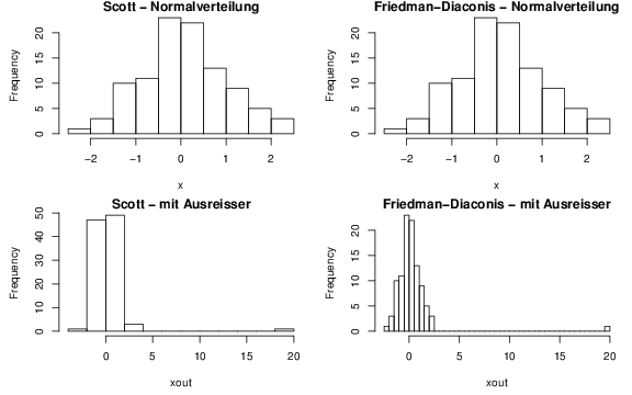
hist(x,breaks="Scott",main="Scott - Normalverteilung")
hist(x,breaks="FD",main="Friedman-Diaconis - Normalverteilung")
hist(xout,breaks="Scott",main="Scott - mit Ausreisser")
hist(xout,breaks="FD",main="Friedman-Diaconis - mit Ausreisser")
dev.off()
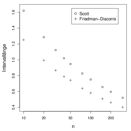
d <- matrix(c(10 , 1.620 , 1.252,
20 , 1.286 , 0.994,
30 , 1.123 , 0.868,
40 , 1.020 , 0.789,
50 , 0.947 , 0.743,
75 , 0.828 , 0.640,
100 , 0.752 , 0.582,
150 , 0.657 , 0.508,
200 , 0.597 , 0.461,
300 , 0.521 , 0.403),ncol=3,byrow=T)
pdf("scottfd.pdf",width=6,height=6)
par(mar=c(4.5,4.5,1,1))
plot(d[,1],d[,2],cex.lab=1.3,log="x",xlab="n",ylab="Intervallänge",ylim=c(0.4,1.65))
points(d[,1],d[,3],pch=3)
legend(52,1.65,c("Scott","Friedman-Diaconis"),pch=c(1,3),cex=1.2)
dev.off()