library(StatDA)
data(AuOLD)
data(AuNEW)
n=length(AuOLD)
pdf("fig-18-7.pdf",width=8,height=7)
par(mfcol=c(2,2),mar=c(4,4,2,2))
###################
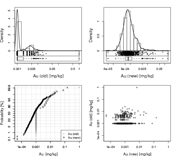
edaplot(log10(AuOLD),H.freq=F,box=T,S.pch=3,S.cex=0.5,D.lwd=1.5,P.ylab="Density",
P.log=T,P.logfine=c(5,10),P.main="",P.xlab="Au (old) [mg/kg]",B.pch=3,B.cex=0.5,
H.breaks=20)
##### QP log
xl=c(min(log10(AuOLD),log10(AuNEW)),max(log10(AuOLD),log10(AuNEW)))
qpplot.das(log10(AuOLD),qdist=qnorm,xlab="Au [mg/kg]", cex.lab=1.2,
ylab="Probability [%]", pch=3,cex=0.7, logx=TRUE,lwd=1.2,line=FALSE,
logfinetick=c(2,5,10),logfinelab=c(10),xlim=xl,col=gray(0.6))
qpplot.das(log10(AuNEW),qdist=qnorm,xlab="Au [mg/kg]", cex.lab=1.2,
ylab="Probability [%]", pch=1,cex=0.7, logx=TRUE,lwd=1.2,line=FALSE,
logfinetick=c(2,5,10),logfinelab=c(10),add.plot=TRUE)
legend("bottomright",pch=c(3,1),pt.cex=c(0.7,0.7),legend=c("Au (old)","Au (new)"),
bg="white",col=c(grey(0.6),1))
###################
edaplot(log10(AuNEW),H.freq=F,box=T,S.pch=3,S.cex=0.5,D.lwd=1.5,P.ylab="Density",
P.log=T,P.logfine=c(5,10),P.main="",P.xlab="Au (new) [mg/kg]",B.pch=3,B.cex=0.5,
H.breaks=20)
###################
lim=c(min(log10(AuNEW),log10(AuOLD)), max(log10(AuNEW),log10(AuOLD)))
plot(log10(AuNEW),log10(AuOLD),xlab="Au (new) [mg/kg]",ylab="Au (old) [mg/kg]",
cex.lab=1.2, cex=0.7, pch=3, xaxt="n", yaxt="n",
xlim=lim, ylim=lim)
axis(1,at=log10(alog<-sort(c((10^(-50:50))%*%t(10)))),labels=alog)
axis(2,at=log10(alog<-sort(c((10^(-50:50))%*%t(10)))),labels=alog)
dev.off()
library(StatDA)
# need data:
data(chorizon)
data(AuOLD)
data(AuNEW)
AuOLD <- AuOLD[-67]
AuNEW <- AuNEW[-67]
pdf("fig-18-8.pdf",width=9,height=4.5)
par(mfcol=c(1,2),mar=c(4,4,2,2))
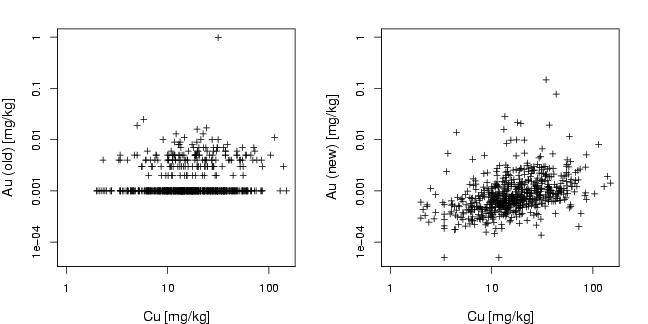
Cu=chorizon[,"Cu"]
lim=c(min(log10(AuOLD),log10(AuNEW)), max(log10(AuOLD),log10(AuNEW)))
plot(log10(Cu),log10(AuOLD),xlab="Cu [mg/kg]",ylab="Au (old) [mg/kg]",
cex.lab=1.2, cex=0.8, pch=3, xaxt="n", yaxt="n", ylim=lim,xlim=c(0,max(log10(Cu))))
axis(1,at=log10(alog<-sort(c((10^(-50:50))%*%t(10)))),labels=alog)
axis(2,at=log10(alog<-sort(c((10^(-50:50))%*%t(10)))),labels=alog)
plot(log10(Cu),log10(AuNEW),xlab="Cu [mg/kg]",ylab="Au (new) [mg/kg]",
cex.lab=1.2, cex=0.8, pch=3, xaxt="n", yaxt="n", ylim=lim,xlim=c(0,max(log10(Cu))))
axis(1,at=log10(alog<-sort(c((10^(-50:50))%*%t(10)))),labels=alog)
axis(2,at=log10(alog<-sort(c((10^(-50:50))%*%t(10)))),labels=alog)
dev.off()
library(StatDA)
# need data:
data(kola.background)
data(chorizon)
data(bordersKola)
data(AuOLD)
data(AuNEW)
X=chorizon[,"XCOO"]
Y=chorizon[,"YCOO"]
xwid=diff(range(X))/12e4
ywid=diff(range(Y))/12e4
pdf("fig-18-9.pdf",width=2*xwid,height=1*ywid)
par(mfrow=c(1,2),mar=c(1.5,1.5,1.5,1.5))
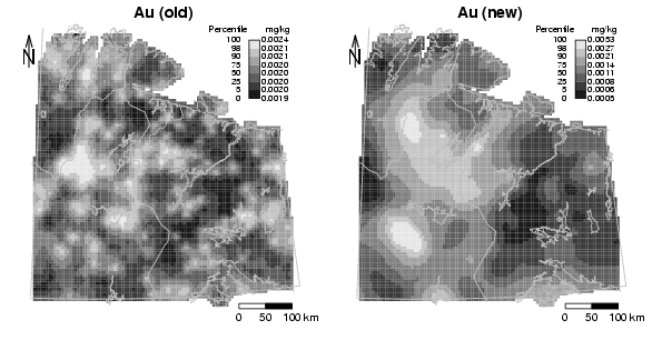
# Au OLD
el=AuOLD[-67]
# Fit variogram for data with non-standardized distance:
v4=variog(coords=cbind(X,Y),data=el,lambda=0,max.dist=200000)
ini.vals <- expand.grid(seq(0,1,l=10), seq(10000,100000,l=10))
v5=variofit(v4,ini.vals,cov.model="matern",max.dist=200000)
# Kriging
# generate plot with packground
plot(X,Y,frame.plot=FALSE,xaxt="n",yaxt="n",xlab="",ylab="",type="n")
KrigeLegend(X,Y,el,resol=100,vario=v5,type="percentile",whichcol="gray",
qutiles=c(0,0.05,0.25,0.50,0.75,0.90,0.98,1),borders="bordersKola",
leg.xpos.min=7.8e5,leg.xpos.max=8.0e5,leg.ypos.min=77.6e5,leg.ypos.max=78.7e5,
leg.title="mg/kg", leg.title.cex=0.7, leg.numb.cex=0.7, leg.round=4,
leg.numb.xshift=0.7e5,leg.perc.xshift=0.4e5,leg.perc.yshift=0.2e5,tit.xshift=0.35e5)
plotbg(map.col=c("gray","gray","gray","gray"),map.lwd=c(1,1,1,1),add.plot=T)
title("Au (old)",cex.main=1.2)
# scalebar
scalebar(761309,7373050,861309,7363050,shifttext=-0.5,shiftkm=37e3,sizetext=0.8)
# North arrow
Northarrow(362602,7818750,362602,7878750,362602,7838750,Alength=0.15,Aangle=15,Alwd=1.3,Tcex=1.6)
# Au NEW
el=AuNEW[-67]
# Fit variogram for data with non-standardized distance:
v4=variog(coords=cbind(X,Y),data=el,lambda=0,max.dist=200000)
# eyefit
###res.eyefit=eyefit(v4)
###dump("res.eyefit","res.eyefit.AuNEW")
data(res.eyefit.AuNEW)
v5=variofit(v4,res.eyefit.AuNEW,cov.model="exponential",max.dist=200000)
# Kriging
# generate plot with packground
plot(X,Y,frame.plot=FALSE,xaxt="n",yaxt="n",xlab="",ylab="",type="n")
KrigeLegend(X,Y,el,resol=100,vario=v5,type="percentile",whichcol="gray",
qutiles=c(0,0.05,0.25,0.50,0.75,0.90,0.98,1),borders="bordersKola",
leg.xpos.min=7.8e5,leg.xpos.max=8.0e5,leg.ypos.min=77.6e5,leg.ypos.max=78.7e5,
leg.title="mg/kg", leg.title.cex=0.7, leg.numb.cex=0.7, leg.round=4,
leg.numb.xshift=0.7e5,leg.perc.xshift=0.4e5,leg.perc.yshift=0.2e5,tit.xshift=0.35e5)
plotbg(map.col=c("gray","gray","gray","gray"),map.lwd=c(1,1,1,1),add.plot=T)
title("Au (new)",cex.main=1.2)
# scalebar
scalebar(761309,7373050,861309,7363050,shifttext=-0.5,shiftkm=37e3,sizetext=0.8)
# North arrow
Northarrow(362602,7818750,362602,7878750,362602,7838750,Alength=0.15,Aangle=15,Alwd=1.3,Tcex=1.6)
dev.off()