# Allocation of observations using robust MCD's
library(StatDA)
data(kola.background)
# DA with vegetation zones
data(ohorizon)
vegzn=ohorizon[,"VEG_ZONE"]
veg=rep(NA,nrow(ohorizon))
veg[vegzn=="BOREAL_FOREST"] <- 1
veg[vegzn=="FOREST_TUNDRA"] <- 2
veg[vegzn=="SHRUB_TUNDRA"] <- 3
veg[vegzn=="DWARF_SHRUB_TUNDRA"] <- 3
veg[vegzn=="TUNDRA"] <- 3
el=c("Ag","Al","As","B","Ba","Bi","Ca","Cd","Co","Cu","Fe","K","Mg","Mn",
"Na","Ni","P","Pb","Rb","S","Sb","Sr","Th","Tl","V","Y","Zn")
x <- log10(ohorizon[!is.na(veg),el])
v <- veg[!is.na(veg)]
X=ohorizon[!is.na(veg),"XCOO"]
Y=ohorizon[!is.na(veg),"YCOO"]
XY=cbind(X,Y)
# true representation of x and y axis of map for plot
xwid=diff(range(X))/12e4
ywid=diff(range(Y))/12e4
pdf("fig-17-6.pdf",width=2*xwid,height=2*ywid)
par(mfrow=c(2,2),mar=c(1.5,1.5,1.5,1.5))
# generate plot with background
plot(X,Y,frame.plot=FALSE,xaxt="n",yaxt="n",xlab="",ylab="",type="n")
plotbg(map.col=c("gray","gray","gray","gray"),add.plot=T)
points(XY[v==1,],pch=3,cex=0.8)
points(XY[v==2,],pch=1,cex=0.8)
points(XY[v==3,],pch=17,cex=0.8)
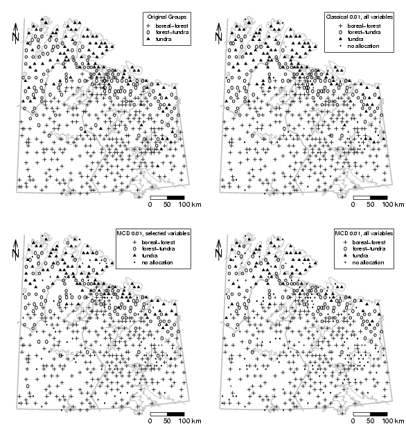
legend("topright",pch=c(3,1,17),pt.cex=c(0.8,0.8,0.8),
legend=c("boreal-forest","forest-tundra","tundra"),
cex=0.8,title="Original Groups")
# scalebar
scalebar(761309,7373050,861309,7363050,shifttext=-0.5,shiftkm=37e3,sizetext=0.8)
# North arrow
Northarrow(362602,7818750,362602,7878750,362602,7838750,Alength=0.15,Aangle=15,Alwd=1.3,Tcex=1.6)
###################################################################################
# Results of Allocation classical 0.01
# Compute results
res.zone1=rg.mva(as.matrix(x[v==1,]))
res.zone2=rg.mva(as.matrix(x[v==2,]))
res.zone3=rg.mva(as.matrix(x[v==3,]))
res=rg.mvalloc(pcrit=0.01,x,res.zone1,res.zone2,res.zone3)
alloc01cla=res$xalloc
# generate plot with background
plot(X,Y,frame.plot=FALSE,xaxt="n",yaxt="n",xlab="",ylab="",type="n")
plotbg(map.col=c("gray","gray","gray","gray"),add.plot=T)
points(XY[alloc01cla==1,],pch=3,cex=0.8,col=1)
points(XY[alloc01cla==2,],pch=1,cex=0.8,col=1)
points(XY[alloc01cla==3,],pch=17,cex=0.8,col=1)
points(XY[alloc01cla==0,],pch=20,cex=0.3,col=1)
legend("topright",pch=c(3,1,17,20),pt.cex=c(0.8,0.8,0.8,0.3),
legend=c("boreal-forest","forest-tundra","tundra","no allocation"),
cex=0.8,title="Classical 0.01, all variables")
# scalebar
scalebar(761309,7373050,861309,7363050,shifttext=-0.5,shiftkm=37e3,sizetext=0.8)
# North arrow
Northarrow(362602,7818750,362602,7878750,362602,7838750,Alength=0.15,Aangle=15,Alwd=1.3,Tcex=1.6)
###################################################################################
# Results of Allocation MCD 0.01 on subset of elements
# Compute results
subvar=c("Ag","B","Bi","Mg","Mn","Na","Pb","Rb","S","Sb","Tl")
set.seed(100)
res.zone1=rg.robmva(as.matrix(x[v==1,subvar]))
res.zone2=rg.robmva(as.matrix(x[v==2,subvar]))
res.zone3=rg.robmva(as.matrix(x[v==3,subvar]))
res=rg.mvalloc(pcrit=0.01,x[,subvar],res.zone1,res.zone2,res.zone3)
alloc01mcd.sub=res$xalloc
# generate plot with background
plot(X,Y,frame.plot=FALSE,xaxt="n",yaxt="n",xlab="",ylab="",type="n")
plotbg(map.col=c("gray","gray","gray","gray"),add.plot=T)
points(XY[alloc01mcd.sub==1,],pch=3,cex=0.8,col=1)
points(XY[alloc01mcd.sub==2,],pch=1,cex=0.8,col=1)
points(XY[alloc01mcd.sub==3,],pch=17,cex=0.8,col=1)
points(XY[alloc01mcd.sub==0,],pch=20,cex=0.3,col=1)
legend("topright",pch=c(3,1,17,20),pt.cex=c(0.8,0.8,0.8,0.3),
legend=c("boreal-forest","forest-tundra","tundra","no allocation"),
cex=0.8,title="MCD 0.01, selected variables")
# scalebar
scalebar(761309,7373050,861309,7363050,shifttext=-0.5,shiftkm=37e3,sizetext=0.8)
# North arrow
Northarrow(362602,7818750,362602,7878750,362602,7838750,Alength=0.15,Aangle=15,Alwd=1.3,Tcex=1.6)
###################################################################################
# Results of Allocation MCD 0.01 on all elements
# Compute results
set.seed(100)
res.zone1=rg.robmva(as.matrix(x[v==1,]))
res.zone2=rg.robmva(as.matrix(x[v==2,]))
res.zone3=rg.robmva(as.matrix(x[v==3,]))
res=rg.mvalloc(pcrit=0.01,x,res.zone1,res.zone2,res.zone3)
alloc01mcd=res$xalloc
# generate plot with background
plot(X,Y,frame.plot=FALSE,xaxt="n",yaxt="n",xlab="",ylab="",type="n")
plotbg(map.col=c("gray","gray","gray","gray"),add.plot=T)
points(XY[alloc01mcd==1,],pch=3,cex=0.8,col=1)
points(XY[alloc01mcd==2,],pch=1,cex=0.8,col=1)
points(XY[alloc01mcd==3,],pch=17,cex=0.8,col=1)
points(XY[alloc01mcd==0,],pch=20,cex=0.3,col=1)
legend("topright",pch=c(3,1,17,20),pt.cex=c(0.8,0.8,0.8,0.3),
legend=c("boreal-forest","forest-tundra","tundra","no allocation"),
cex=0.8,title="MCD 0.01, all variables")
# scalebar
scalebar(761309,7373050,861309,7363050,shifttext=-0.5,shiftkm=37e3,sizetext=0.8)
# North arrow
Northarrow(362602,7818750,362602,7878750,362602,7838750,Alength=0.15,Aangle=15,Alwd=1.3,Tcex=1.6)
dev.off()
table(alloc01cla,v)
table(alloc01mcd.sub,v)
table(alloc01mcd,v)