17.4 Prediction With Discriminant Analysis

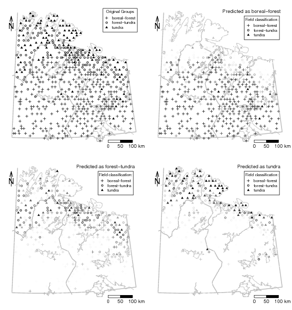
# Fig. 17.3.: Robust QDA for 3 vegetation zones library(StatDA) data(kola.background) # DA with vegetation zones data(ohorizon) vegzn=ohorizon[,"VEG_ZONE"] veg=rep(NA,nrow(ohorizon)) veg[vegzn=="BOREAL_FOREST"] <- 1 veg[vegzn=="FOREST_TUNDRA"] <- 2 veg[vegzn=="SHRUB_TUNDRA"] <- 3 veg[vegzn=="DWARF_SHRUB_TUNDRA"] <- 3 veg[vegzn=="TUNDRA"] <- 3 #el=c("Ag","B","Bi","Ca_AA","Cd","Cu","Fe_AA","K_AA","Mg_AA","Mn_AA","Pb") #el=c("Ag","B","Bi","Ca_AA","Cd","Cu","Fe_AA","K_AA","Mg_AA","Mn_AA","Pb") #el=c("Al_AA","Ba_AA","Ca_AA","Co_AA","Cu_AA","Fe_AA","K_AA","Mg_AA","Mn_AA", # "Ni_AA","S_AA","SR_AA","Zn_AA") el=c("Ag","Al","As","B","Ba","Bi","Ca","Cd","Co","Cu","Fe","K","Mg","Mn", "Na","Ni","P","Pb","Rb","S","Sb","Sr","Th","Tl","V","Y","Zn") ##el=c("Ag","Al","As","Ba","Bi","Ca","Cd","Co","Cu","Fe","K","Mn", ## "Ni","P","Pb","Rb","Sb","Th","Tl","V","Y","Zn") x <- log10(ohorizon[!is.na(veg),el]) #x <- log10(ohorizon[!is.na(veg),c(14:17,19:32,34:61,64,66:85)]) #x=scale(x) v <- veg[!is.na(veg)] X=ohorizon[!is.na(veg),"XCOO"] Y=ohorizon[!is.na(veg),"YCOO"] XY=cbind(X,Y) # true representation of x and y axis of map for plot xwid=diff(range(X))/12e4 ywid=diff(range(Y))/12e4 pdf("fig-17-3.pdf",width=2*xwid,height=2*ywid) par(mfrow=c(2,2),mar=c(1.5,1.5,1.5,1.5)) # generate plot with background plot(X,Y,frame.plot=FALSE,xaxt="n",yaxt="n",xlab="",ylab="",type="n") plotbg(map.col=c("gray","gray","gray","gray"),add.plot=T) points(XY[v==1,],pch=3,cex=0.8) points(XY[v==2,],pch=1,cex=0.8) points(XY[v==3,],pch=17,cex=0.8) set.seed(201) #x.rqda=qda(x, v, subset=train, method="mve") #x.rqda=lda(x, v, subset=train) x.rqda=lda(x, v, CV=TRUE) #x.rqda.pred=predict(x.rqda,x) cl=x.rqda$class pt=x.rqda$post pt.na=apply(is.na(pt),1,sum) cl.red=cl[pt.na==0] pt.red=pt[pt.na==0,] legend("topright",pch=c(3,1,17),pt.cex=c(0.8,0.8,0.8), legend=c("boreal-forest","forest-tundra","tundra"), cex=0.8,title="Original Groups") # scalebar scalebar(761309,7373050,861309,7363050,shifttext=-0.5,shiftkm=37e3,sizetext=0.8) # North arrow Northarrow(362602,7818750,362602,7878750,362602,7838750,Alength=0.15,Aangle=15,Alwd=1.3,Tcex=1.6) ################################################################################### # Results Group 1 # generate plot with background plot(X,Y,frame.plot=FALSE,xaxt="n",yaxt="n",xlab="",ylab="",type="n") plotbg(map.col=c("gray","gray","gray","gray"),add.plot=T) #points(XY,pch=15,cex=0.6,col=gray(1-pt.red[,1])) v.red=v[pt.na==0] XY.red=XY[pt.na==0,] points(XY.red[v.red==1,],pch=3,cex=0.8,col=gray(1-pt.red[v.red==1,1])) points(XY.red[v.red==2,],pch=1,cex=0.8,col=gray(1-pt.red[v.red==2,1])) points(XY.red[v.red==3,],pch=17,cex=0.8,col=gray(1-pt.red[v.red==3,1])) #points(XY[cl.red==1,],pch=15,cex=0.6,col=gray(1-pt.red[cl.red==1,1])) #points(XY[cl.red==2,],pch=1,cex=0.6,col=gray(1-pt.red[cl.red==2,2])) #points(XY[cl.red==3,],pch=17,cex=0.6,col=gray(1-pt.red[cl.red==3,3])) text(750000,7900000,"Predicted as boreal-forest",cex=1) legend(720000,7880000,pch=c(3,1,17),pt.cex=c(0.8,0.8,0.8), legend=c("boreal-forest","forest-tundra","tundra"), cex=0.8,title="Field classification:") # scalebar scalebar(761309,7373050,861309,7363050,shifttext=-0.5,shiftkm=37e3,sizetext=0.8) # North arrow Northarrow(362602,7818750,362602,7878750,362602,7838750,Alength=0.15,Aangle=15,Alwd=1.3,Tcex=1.6) ################################################################################### # Results Group 2 # generate plot with background plot(X,Y,frame.plot=FALSE,xaxt="n",yaxt="n",xlab="",ylab="",type="n") plotbg(map.col=c("gray","gray","gray","gray"),add.plot=T) #points(XY,pch=15,cex=0.6,col=gray(1-pt.red[,1])) v.red=v[pt.na==0] XY.red=XY[pt.na==0,] points(XY.red[v.red==1,],pch=3,cex=0.8,col=gray(1-pt.red[v.red==1,2])) points(XY.red[v.red==2,],pch=1,cex=0.8,col=gray(1-pt.red[v.red==2,2])) points(XY.red[v.red==3,],pch=17,cex=0.8,col=gray(1-pt.red[v.red==3,2])) #points(XY[cl.red==1,],pch=15,cex=0.6,col=gray(1-pt.red[cl.red==1,1])) #points(XY[cl.red==2,],pch=1,cex=0.6,col=gray(1-pt.red[cl.red==2,2])) #points(XY[cl.red==3,],pch=17,cex=0.6,col=gray(1-pt.red[cl.red==3,3])) text(750000,7900000,"Predicted as forest-tundra",cex=1) legend(720000,7880000,pch=c(3,1,17),pt.cex=c(0.8,0.8,0.8), legend=c("boreal-forest","forest-tundra","tundra"), cex=0.8,title="Field classification:") # scalebar scalebar(761309,7373050,861309,7363050,shifttext=-0.5,shiftkm=37e3,sizetext=0.8) # North arrow Northarrow(362602,7818750,362602,7878750,362602,7838750,Alength=0.15,Aangle=15,Alwd=1.3,Tcex=1.6) ################################################################################### # Results Group 3 # generate plot with background plot(X,Y,frame.plot=FALSE,xaxt="n",yaxt="n",xlab="",ylab="",type="n") plotbg(map.col=c("gray","gray","gray","gray"),add.plot=T) #points(XY,pch=15,cex=0.6,col=gray(1-pt.red[,1])) v.red=v[pt.na==0] XY.red=XY[pt.na==0,] points(XY.red[v.red==1,],pch=3,cex=0.8,col=gray(1-pt.red[v.red==1,3])) points(XY.red[v.red==2,],pch=1,cex=0.8,col=gray(1-pt.red[v.red==2,3])) points(XY.red[v.red==3,],pch=17,cex=0.8,col=gray(1-pt.red[v.red==3,3])) #points(XY[cl.red==1,],pch=15,cex=0.6,col=gray(1-pt.red[cl.red==1,1])) #points(XY[cl.red==2,],pch=1,cex=0.6,col=gray(1-pt.red[cl.red==2,2])) #points(XY[cl.red==3,],pch=17,cex=0.6,col=gray(1-pt.red[cl.red==3,3])) text(780000,7900000,"Predicted as tundra",cex=1) legend(720000,7880000,pch=c(3,1,17),pt.cex=c(0.8,0.8,0.8), legend=c("boreal-forest","forest-tundra","tundra"), cex=0.8,title="Field classification:") # scalebar scalebar(761309,7373050,861309,7363050,shifttext=-0.5,shiftkm=37e3,sizetext=0.8) # North arrow Northarrow(362602,7818750,362602,7878750,362602,7838750,Alength=0.15,Aangle=15,Alwd=1.3,Tcex=1.6) ################################################################################### a1=sum(cl[v==1]!=v[v==1]) a2=sum(cl[v==2]!=v[v==2]) a3=sum(cl[v==3]!=v[v==3]) b1=a1/sum(v==1)*100 b2=a2/sum(v==2)*100 b3=a3/sum(v==3)*100 print(c(b1,b2,b3,(a1+a2+a3)/length(v)*100)) dev.off()

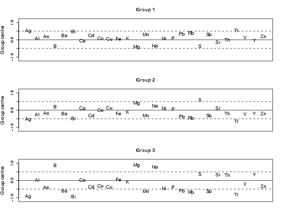
# Fig. 17.4.: Robust QDA for 3 vegetation zones library(StatDA) # DA with vegetation zones data(ohorizon) vegzn=ohorizon[,"VEG_ZONE"] veg=rep(NA,nrow(ohorizon)) veg[vegzn=="BOREAL_FOREST"] <- 1 veg[vegzn=="FOREST_TUNDRA"] <- 2 veg[vegzn=="SHRUB_TUNDRA"] <- 3 veg[vegzn=="DWARF_SHRUB_TUNDRA"] <- 3 veg[vegzn=="TUNDRA"] <- 3 el=c("Ag","Al","As","B","Ba","Bi","Ca","Cd","Co","Cu","Fe","K","Mg","Mn", "Na","Ni","P","Pb","Rb","S","Sb","Sr","Th","Tl","V","Y","Zn") x <- log10(ohorizon[!is.na(veg),el]) x=scale(x) v <- veg[!is.na(veg)] pdf("fig-17-4.pdf",width=8,height=6) par(mfrow=c(1,1),mar=c(2,2,2,2)) set.seed(201) #x.rqda=qda(x, v, subset=train, method="mve") #x.rqda=lda(x, v, subset=train) x.da=lda(x, v) x.da.pred=predict(x.da,x) cl=x.da.pred$cl plotelement(x.da) ################################################################################### a1=sum(cl[v==1]!=v[v==1]) a2=sum(cl[v==2]!=v[v==2]) a3=sum(cl[v==3]!=v[v==3]) b1=a1/sum(v==1)*100 b2=a2/sum(v==2)*100 b3=a3/sum(v==3)*100 print(c(b1,b2,b3,(a1+a2+a3)/length(v)*100)) dev.off()