library(StatDA)
data(chorizon)
x=log10(chorizon[,c("Cr","K")])
lit=chorizon[,"LITO"]
Region=rep(1, length(lit))
Region[lit==10] <- 3
pdf("fig-17-1.pdf",width=9,height=4.5)
par(mfcol=c(1,2),mar=c(4,4,2,2))
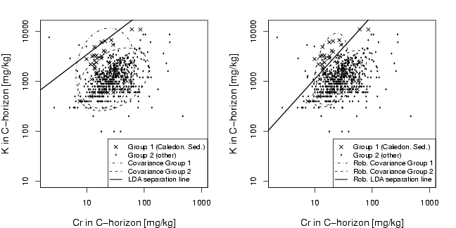
plot(x,xlab="Cr in C-horizon [mg/kg]",ylab="K in C-horizon [mg/kg]",
cex.lab=1.2, cex=0.7, pch=3, xaxt="n", yaxt="n",type="n",
xlim=c(0.3,3),ylim=c(1,4.1))
axis(1,at=log10(alog<-sort(c((10^(-50:50))%*%t(c(10))))),labels=alog)
axis(2,at=log10(alog<-sort(c((10^(-50:50))%*%t(c(10))))),labels=alog)
points(x[Region==1,],pch=1,cex=0.2)
points(x[Region==3,],pch=4,cex=0.9)
###############################################################################
# construct LDA line:
x1=x[Region==1,]
x3=x[Region==3,]
n1=nrow(x1)
n3=nrow(x3)
p1=n1/(n1+n3)
p3=n3/(n1+n3)
m1=apply(x1,2,mean)
m3=apply(x3,2,mean)
S1=cov(x1)
S3=cov(x3)
Sp=((n1-1)/(n1-1+n3-1))*S1+((n3-1)/(n1-1+n3-1))*S3
Sp1=solve(Sp)
y=x
yLDA=as.numeric(t(m1-m3)%*%Sp1%*%t(y)-as.numeric(1/2*t(m1-m3)%*%Sp1%*%(m1+m3)))-log(p3/p1)
#plot(yLDA,col=as.numeric(x.lda.pred$class))
#abline(h=0)
# Misclassification:
yLDAclass=(yLDA<0)
# LDA
y1=seq(from=min(x[,1])-0.2,to=max(x[,1]),by=0.005)
y2=seq(from=min(x[,2]),to=max(x[,2])+0.2,by=0.005)
y1a=rep(y1,length(y2))
y2a=sort(rep(y2,length(y1)))
#points(y1a,y2a,col=2,cex=0.2)
ya=cbind(y1a,y2a)
yaLDA=as.numeric(t(m1-m3)%*%Sp1%*%t(ya)-
as.numeric(1/2*t(m1-m3)%*%Sp1%*%(m1+m3)))-log(p3/p1)
#plot(log10(chorizon[,"Cr"]),log10(chorizon[,"K"]),pch=Region,cex=Region/3+0.3)
#points(y1a[yaLDA<0],y2a[yaLDA<0],col=3,cex=0.2)
#points(y1a[yaLDA>0],y2a[yaLDA>0],col=2,cex=0.2)
#points(log10(chorizon[,"Cr"]),log10(chorizon[,"K"]),pch=Region,cex=Region/3+0.3)
boundLDA=abs(yaLDA)<0.01
lines(lowess(y1a[boundLDA],y2a[boundLDA]),col=1,lwd=1.5,lty=1)
plotellipse(m1,S1,perc=c(0.9),lty=c(2,2))
plotellipse(m3,S3,perc=c(0.9),lty=c(4,4))
legend("bottomright",legend=c("Group 1 (Caledon. Sed.)","Group 2 (other)",
"Covariance Group 1", "Covariance Group 2",
"LDA separation line"),
pch=c(4,1,NA,NA,NA),lty=c(NA,NA,4,2,1),lwd=c(NA,NA,1,1,1.5),
pt.cex=c(0.9,0.2,NA,NA,NA),cex=0.8)
###############################################################################
# construct robust LDA line:
plot(x,xlab="Cr in C-horizon [mg/kg]",ylab="K in C-horizon [mg/kg]",
cex.lab=1.2, cex=0.7, pch=3, xaxt="n", yaxt="n",type="n",
xlim=c(0.3,3),ylim=c(1,4.1))
axis(1,at=log10(alog<-sort(c((10^(-50:50))%*%t(c(10))))),labels=alog)
axis(2,at=log10(alog<-sort(c((10^(-50:50))%*%t(c(10))))),labels=alog)
points(x[Region==1,],pch=1,cex=0.2)
points(x[Region==3,],pch=4,cex=0.9)
# Robust:
x1=x[Region==1,]
x3=x[Region==3,]
n1=nrow(x1)
n3=nrow(x3)
p1=n1/(n1+n3)
p3=n3/(n1+n3)
set.seed(100)
x1.mve=cov.mve(x1)
m1=x1.mve$cen
S1=cov.mve(x1)$cov
set.seed(100)
x3.mve=cov.mve(x3)
m3=x3.mve$cen
S3=cov.mve(x3)$cov
Sp=((n1-1)/(n1-1+n3-1))*S1+((n3-1)/(n1-1+n3-1))*S3
Sp1=solve(Sp)
y=x
yLDA=as.numeric(t(m1-m3)%*%Sp1%*%t(y)-as.numeric(1/2*t(m1-m3)%*%Sp1%*%(m1+m3)))-log(p3/p1)
#plot(yLDA,col=as.numeric(x.lda.pred$class))
#abline(h=0)
# Misclassification:
yRLDAclass=(yLDA<0)
# LDA
y1=seq(from=min(x[,1])-0.2,to=max(x[,1]),by=0.005)
y2=seq(from=min(x[,2]),to=max(x[,2])+0.2,by=0.005)
y1a=rep(y1,length(y2))
y2a=sort(rep(y2,length(y1)))
#points(y1a,y2a,col=2,cex=0.2)
ya=cbind(y1a,y2a)
yaLDA=as.numeric(t(m1-m3)%*%Sp1%*%t(ya)-
as.numeric(1/2*t(m1-m3)%*%Sp1%*%(m1+m3)))-log(p3/p1)
#plot(log10(chorizon[,"Cr"]),log10(chorizon[,"K"]),pch=Region,cex=Region/3+0.3)
#points(y1a[yaLDA<0],y2a[yaLDA<0],col=3,cex=0.2)
#points(y1a[yaLDA>0],y2a[yaLDA>0],col=2,cex=0.2)
#points(log10(chorizon[,"Cr"]),log10(chorizon[,"K"]),pch=Region,cex=Region/3+0.3)
boundLDA=abs(yaLDA)<0.01
lines(lowess(y1a[boundLDA],y2a[boundLDA]),col=1,lwd=1.5,lty=1)
plotellipse(m1,S1,perc=c(0.9),lty=c(2,2))
plotellipse(m3,S3,perc=c(0.9),lty=c(4,4))
legend("bottomright",legend=c("Group 1 (Caledon. Sed.)","Group 2 (other)",
"Rob. Covariance Group 1", "Rob. Covariance Group 2",
"Rob. LDA separation line"),
pch=c(4,1,NA,NA,NA),lty=c(NA,NA,4,2,1),lwd=c(NA,NA,1,1,1.5),
pt.cex=c(0.9,0.2,NA,NA,NA),cex=0.8)
dev.off()
### print(t(table(yLDAclass,Region)))
### print(table(Region,yLDAclass)/as.vector(table(Region))*100)
### print(t(table(yRLDAclass,Region)))
### print(table(Region,yRLDAclass)/as.vector(table(Region))*100)
library(StatDA)
data(chorizon)
x=log10(chorizon[,c("Cr","K")])
lit=chorizon[,"LITO"]
Region=rep(1, length(lit))
Region[lit==10] <- 3
pdf("fig-17-2.pdf",width=9,height=4.5)
par(mfcol=c(1,2),mar=c(4,4,2,2))
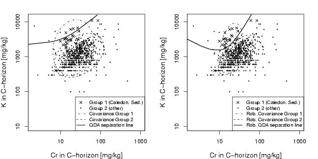
plot(x,xlab="Cr in C-horizon [mg/kg]",ylab="K in C-horizon [mg/kg]",
cex.lab=1.2, cex=0.7, pch=3, xaxt="n", yaxt="n",type="n",
xlim=c(0.3,3),ylim=c(1,4.1))
axis(1,at=log10(alog<-sort(c((10^(-50:50))%*%t(c(10))))),labels=alog)
axis(2,at=log10(alog<-sort(c((10^(-50:50))%*%t(c(10))))),labels=alog)
points(x[Region==1,],pch=1,cex=0.2)
points(x[Region==3,],pch=4,cex=0.9)
###############################################################################
# construct QDA line:
x1=x[Region==1,]
x3=x[Region==3,]
n1=nrow(x1)
n3=nrow(x3)
p1=n1/(n1+n3)
p3=n3/(n1+n3)
m1=apply(x1,2,mean)
m3=apply(x3,2,mean)
S1=cov(x1)
S3=cov(x3)
Sp=((n1-1)/(n1-1+n3-1))*S1+((n3-1)/(n1-1+n3-1))*S3
Sp1=solve(Sp)
S1m=solve(S1)
S3m=solve(S3)
y=x
yQDA = as.vector(-1/2*diag(as.matrix(y)%*%(S1m-S3m)%*%t(y)))+
as.vector((t(m1)%*%S1m-t(m3)%*%S3m)%*%t(y))-
( 1/2*log(det(S1)/det(S3))+
as.numeric(1/2*(t(m1)%*%S1m%*%m1))-
as.numeric(1/2*(t(m3)%*%S3m%*%m3)))-log(p3/p1)
#plot(yQDA,col=as.numeric(x.qda.pred$class))
#abline(h=0)
# Misclassification:
yQDAclass=(yQDA<0)
# QDA
y1=seq(from=min(x[,1])-0.2,to=max(x[,1]),by=0.005)
y2=seq(from=min(x[,2])+1,to=max(x[,2])+0.2,by=0.005)
y1a=rep(y1,length(y2))
y2a=sort(rep(y2,length(y1)))
#points(y1a,y2a,col=2,cex=0.2)
ya=cbind(y1a,y2a)
yaQDA =-1/2*apply((as.matrix(ya)%*%(S1m-S3m))*as.matrix((ya)),1,sum)+
as.vector((t(m1)%*%S1m-t(m3)%*%S3m)%*%t(ya))-
( 1/2*log(det(S1)/det(S3))+
as.numeric(1/2*(t(m1)%*%S1m%*%m1))-
as.numeric(1/2*(t(m3)%*%S3m%*%m3)))-log(p3/p1)
#plot(log10(chorizon[,"Cr"]),log10(chorizon[,"K"]),pch=Region,cex=Region/3+0.3)
#points(y1a[yaQDA<0],y2a[yaQDA<0],col=3,cex=0.2)
#points(y1a[yaQDA>0],y2a[yaQDA>0],col=2,cex=0.2)
#points(log10(chorizon[,"Cr"]),log10(chorizon[,"K"]),pch=Region,cex=Region/3+0.3)
boundQDA=abs(yaQDA)<0.01
lines(lowess(y1a[boundQDA],y2a[boundQDA]),col=1,lwd=1.5,lty=1)
plotellipse(m1,S1,perc=c(0.9),lty=c(2,2))
plotellipse(m3,S3,perc=c(0.9),lty=c(4,4))
legend("bottomright",legend=c("Group 1 (Caledon. Sed.)","Group 2 (other)",
"Covariance Group 1", "Covariance Group 2",
"QDA separation line"),
pch=c(4,1,NA,NA,NA),lty=c(NA,NA,4,2,1),lwd=c(NA,NA,1,1,1.5),
pt.cex=c(0.9,0.2,NA,NA,NA),cex=0.8)
###############################################################################
# construct robust QDA line:
plot(x,xlab="Cr in C-horizon [mg/kg]",ylab="K in C-horizon [mg/kg]",
cex.lab=1.2, cex=0.7, pch=3, xaxt="n", yaxt="n",type="n",
xlim=c(0.3,3),ylim=c(1,4.1))
axis(1,at=log10(alog<-sort(c((10^(-50:50))%*%t(c(10))))),labels=alog)
axis(2,at=log10(alog<-sort(c((10^(-50:50))%*%t(c(10))))),labels=alog)
points(x[Region==1,],pch=1,cex=0.2)
points(x[Region==3,],pch=4,cex=0.9)
# Robust:
x1=x[Region==1,]
x3=x[Region==3,]
n1=nrow(x1)
n3=nrow(x3)
p1=n1/(n1+n3)
p3=n3/(n1+n3)
set.seed(100)
x1.mve=cov.mve(x1)
m1=x1.mve$cen
S1=cov.mve(x1)$cov
set.seed(100)
x3.mve=cov.mve(x3)
m3=x3.mve$cen
S3=cov.mve(x3)$cov
Sp=((n1-1)/(n1-1+n3-1))*S1+((n3-1)/(n1-1+n3-1))*S3
Sp1=solve(Sp)
y=x
# QDA
S1m=solve(S1)
S3m=solve(S3)
yQDA = as.vector(-1/2*diag(as.matrix(y)%*%(S1m-S3m)%*%t(y)))+
as.vector((t(m1)%*%S1m-t(m3)%*%S3m)%*%t(y))-
( 1/2*log(det(S1)/det(S3))+
as.numeric(1/2*(t(m1)%*%S1m%*%m1))-
as.numeric(1/2*(t(m3)%*%S3m%*%m3)))-log(p3/p1)
#plot(yQDA,col=as.numeric(x.qda.pred$class))
#abline(h=0)
# Misclassification:
yRQDAclass=(yQDA<0)
y1=seq(from=min(x[,1]-0.2),to=max(x[,1]),by=0.005)
y2=seq(from=min(x[,2]+1),to=max(x[,2]+0.2),by=0.005)
y1a=rep(y1,length(y2))
y2a=sort(rep(y2,length(y1)))
#points(y1a,y2a,col=2,cex=0.2)
ya=cbind(y1a,y2a)
yaQDA =-1/2*apply((as.matrix(ya)%*%(S1m-S3m))*as.matrix((ya)),1,sum)+
as.vector((t(m1)%*%S1m-t(m3)%*%S3m)%*%t(ya))-
( 1/2*log(det(S1)/det(S3))+
as.numeric(1/2*(t(m1)%*%S1m%*%m1))-
as.numeric(1/2*(t(m3)%*%S3m%*%m3)))-log(p3/p1)
#plot(log10(chorizon[,"Cr"]),log10(chorizon[,"K"]),pch=Region,cex=Region/3+0.3)
#points(y1a[yaQDA<0],y2a[yaQDA<0],col=3,cex=0.2)
#points(y1a[yaQDA>0],y2a[yaQDA>0],col=2,cex=0.2)
#points(log10(chorizon[,"Cr"]),log10(chorizon[,"K"]),pch=Region,cex=Region/3+0.3)
boundQDA=abs(yaQDA)<0.01
low=lowess(y1a[boundQDA],y2a[boundQDA],f=0.3)
lines(low$x,low$y,col=1,lwd=1.5,lty=1)
plotellipse(m1,S1,perc=c(0.9),lty=c(2,2))
plotellipse(m3,S3,perc=c(0.9),lty=c(4,4))
legend("bottomright",legend=c("Group 1 (Caledon. Sed.)","Group 2 (other)",
"Rob. Covariance Group 1", "Rob. Covariance Group 2",
"Rob. QDA separation line"),
pch=c(4,1,NA,NA,NA),lty=c(NA,NA,4,2,1),lwd=c(NA,NA,1,1,1.5),
pt.cex=c(0.9,0.2,NA,NA,NA),cex=0.8)
dev.off()
### print(t(table(yQDAclass,Region)))
### print(table(Region,yQDAclass)/as.vector(table(Region))*100)
### print(t(table(yRQDAclass,Region)))
### print(table(Region,yRQDAclass)/as.vector(table(Region))*100)