16.2 Multiple Regression

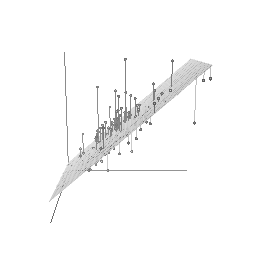
# Fig. 16.5.: Illustration of multiple lin. and quadr. Regression # ATTENTION: this script file does not automatically generate the pdf figure # We used other graphics programs to make the figure nice! library(StatDA) data(chorizon) attach(chorizon) lit=1 scatter3dPETER(x=log10(chorizon[chorizon$LITO==lit,"Cr"]), z=log10(chorizon[chorizon$LITO==lit,"Cr_INAA"]), y=log10(chorizon[chorizon$LITO==lit,"Co"]), ##xlab="Cr", zlab="Cr_INAA", ylab="Co", xlab="",ylab="",zlab="", neg.res.col=gray(0.6), pos.res.col=gray(0.1), point.col=1, fov=30, surface.col="black",grid.col="gray",sphere.size=0.8) rgl.snapshot("fig-16-5a.png",fmt="png") rgl.close() 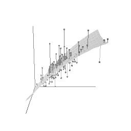lit=1 scatter3dPETER(x=log10(chorizon[chorizon$LITO==lit,"Cr"]), z=log10(chorizon[chorizon$LITO==lit,"Cr_INAA"]), y=log10(chorizon[chorizon$LITO==lit,"Co"]), ##xlab="Cr", zlab="Cr_INAA", ylab="Co", xlab="",ylab="",zlab="", neg.res.col=gray(0.6), pos.res.col=gray(0.1), point.col=1, fov=30, surface.col="black",grid.col="gray",sphere.size=0.8, fit="quadratic") rgl.snapshot("fig-16-5b.png",fmt="png") rgl.close()