library(StatDA)
pdf("fig-16-1.pdf",width=9,height=4.5)
par(mfrow=c(1,2),mar=c(4,4,2,2))
data(chorizon)
coun=chorizon[,"COUN"]
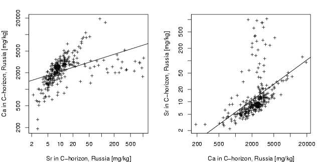
Sr=chorizon[coun=="RUS","Sr"]
Ca=chorizon[coun=="RUS","Ca"]
plot(log10(Sr),log10(Ca),xlab="Sr in C-horizon, Russia [mg/kg]",
ylab="Ca in C-horizon, Russia [mg/kg]", pch=3, cex=0.7, cex.lab=1,xaxt="n",
yaxt="n")
axis(1,at=log10(a<-sort(c((10^(-50:50))%*%t(c(2,5,10))))),labels=a)
axis(2,at=log10(a<-sort(c((10^(-50:50))%*%t(c(2,5,10))))),labels=a)
abline(lsfit(log10(Sr),log10(Ca)))
plot(log10(Ca),log10(Sr),xlab="Ca in C-horizon, Russia [mg/kg]",
ylab="Sr in C-horizon, Russia [mg/kg]", pch=3, cex=0.7, cex.lab=1,xaxt="n",
yaxt="n")
axis(1,at=log10(a<-sort(c((10^(-50:50))%*%t(c(2,5,10))))),labels=a)
axis(2,at=log10(a<-sort(c((10^(-50:50))%*%t(c(2,5,10))))),labels=a)
abline(lsfit(log10(Ca),log10(Sr)))
dev.off()
library(StatDA)
data(moss)
Cu=moss[,"Cu"]
Ni=moss[,"Ni"]
pdf("fig-16-2.pdf",width=9,height=4.5)
# randomly select N points
par(mfrow=c(1,2),mar=c(4,4,2,2))
N=50
set.seed(106)
Nsel=sample(1:length(Cu),N)
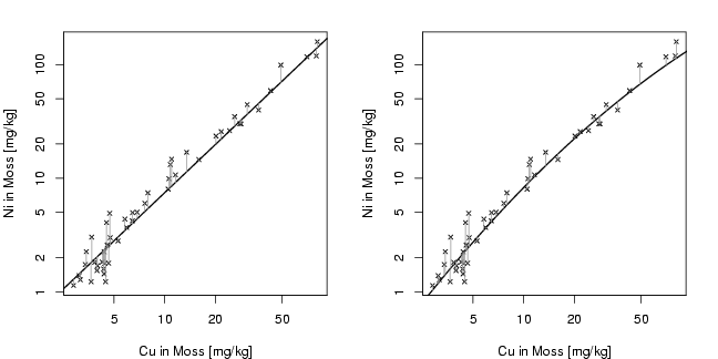
Cu.sel=log10(Cu[Nsel])
Ni.sel=log10(Ni[Nsel])
plot(Cu.sel,Ni.sel,xlab="Cu in Moss [mg/kg]",
ylab="Ni in Moss [mg/kg]", pch=4, cex=0.7, cex.lab=1,xaxt="n",
yaxt="n")
axis(1,at=log10(a<-sort(c((10^(-50:50))%*%t(c(2,5,10))))),labels=a)
axis(2,at=log10(a<-sort(c((10^(-50:50))%*%t(c(2,5,10))))),labels=a)
lm1=lm(log10(Ni)~log10(Cu))
abline(lm1,lty=1,lwd=1.5)
lm1.pred=predict.lm(lm1)[Nsel]
for (i in 1:N){
segments(Cu.sel[i],lm1.pred[i],Cu.sel[i],Ni.sel[i],col=gray(0.6))
}
plot(Cu.sel,Ni.sel,xlab="Cu in Moss [mg/kg]",
ylab="Ni in Moss [mg/kg]", pch=4, cex=0.7, cex.lab=1,xaxt="n",
yaxt="n")
axis(1,at=log10(a<-sort(c((10^(-50:50))%*%t(c(2,5,10))))),labels=a)
axis(2,at=log10(a<-sort(c((10^(-50:50))%*%t(c(2,5,10))))),labels=a)
lm2=lm(log10(Ni)~log10(Cu)+I((log10(Cu))^2))
ind=sort(Cu,index.return=T)$ix
lines(log10(Cu[ind]),predict.lm(lm2)[ind],lwd=1.5)
lm2.pred=predict.lm(lm2)[Nsel]
for (i in 1:N){
segments(Cu.sel[i],lm2.pred[i],Cu.sel[i],Ni.sel[i],col=gray(0.6))
}
dev.off()
library(StatDA)
data(moss)
Cu=moss[,"Cu"]
Ni=moss[,"Ni"]
data(kola.background)
X=moss[,"XCOO"]
Y=moss[,"YCOO"]
# true representation of x and y axis of map for plot
xwid=diff(range(X))/12e4
ywid=diff(range(Y))/12e4
pdf("fig-16-3.pdf",width=2*xwid,height=1*ywid)
par(mfrow=c(1,2),mar=c(4,4,2,2))
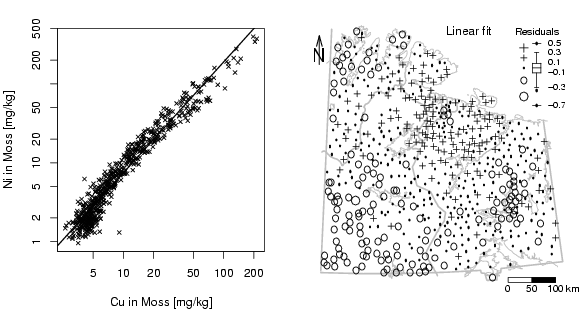
plot(log10(Cu),log10(Ni),xlab="Cu in Moss [mg/kg]",
ylab="Ni in Moss [mg/kg]", pch=4, cex=0.7, cex.lab=1,xaxt="n",
yaxt="n")
axis(1,at=log10(a<-sort(c((10^(-50:50))%*%t(c(2,5,10))))),labels=a)
axis(2,at=log10(a<-sort(c((10^(-50:50))%*%t(c(2,5,10))))),labels=a)
lm1=lm(log10(Ni)~log10(Cu))
abline(lm1,lty=1,lwd=1.5)
### NEW MAP:
par(mar=c(1.5,1.5,1.5,1.5))
dat=lm1$res
boxinfo=boxplot(dat,plot=F)
# generate plot with packground
plot(X,Y,frame.plot=FALSE,xaxt="n",yaxt="n",xlab="",ylab="",type="n")
plotbg(map.col=c("gray","gray","gray","gray"),add.plot=T)
SymbLegend(X,Y,dat,type="boxplot",qutiles<-c(0,0.05,0.25,0.75,0.95,1),symbtype="EDA",symbmagn=0.8,
leg.position="topright",leg.title="Residuals",leg.title.cex=0.8,leg.round=4,leg.wid=7,
leg.just="right",cex.scale=0.75,xf=9e3,logscale=FALSE,accentuate=FALSE)
# Class legend
text(min(X)+diff(range(X))*5/8,max(Y),"Linear fit",cex=1.0)
# scalebar
scalebar(761309,7373050,861309,7363050,shifttext=-0.5,shiftkm=37e3,sizetext=0.8)
# North arrow
Northarrow(362602,7818750,362602,7878750,362602,7838750,Alength=0.15,Aangle=15,Alwd=1.3,Tcex=1.6)
dev.off()