15.3.2 Partitioning Methods

# Fig. 15.3.: kmeans and PAM library(StatDA) data(chorizon) data(kola.background) el=c("Na","Ca","K","Al") x=chorizon[,el] sel=((chorizon[,"LITO"]==9) | (chorizon[,"LITO"]==82)) x=scale(log10(x[sel,])) lab=chorizon[sel,"LITO"] lab.new=lab lab.new[lab==82] <- 1 lab.new[lab==9] <- 3 set.seed(100) res2=kmeans(x,2) res2cl=res2$cl+2 res2cl[res2cl==4] <- 1 set.seed(100) res3=pam(x,2,metric="manhattan") res3cl=res3$cluster+2 res3cl[res3cl==4] <- 1 X=chorizon[,"XCOO"] Y=chorizon[,"YCOO"] # true representation of x and y axis of map for plot xwid=diff(range(X))/12e4 ywid=diff(range(Y))/12e4 pdf("fig-15-3.pdf",width=2*xwid,height=1*ywid) par(mfrow=c(1,2),mar=c(1.5,1.5,1.5,1.5)) # NEW MAP plot(X,Y,frame.plot=FALSE,xaxt="n",yaxt="n",xlab="",ylab="",type="n") plotbg(map.col=c("gray","gray","gray","gray"),add.plot=T) 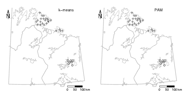points(chorizon[sel,"XCOO"],chorizon[sel,"YCOO"],col=1,pch=res2cl) # Legend text(752000,7880000,"k-means",cex=1) # scalebar scalebar(761309,7373050,861309,7363050,shifttext=-0.5,shiftkm=37e3,sizetext=0.8) # North arrow Northarrow(362602,7818750,362602,7878750,362602,7838750,Alength=0.15,Aangle=15,Alwd=1.3,Tcex=1.6) # NEW MAP plot(X,Y,frame.plot=FALSE,xaxt="n",yaxt="n",xlab="",ylab="",type="n") plotbg(map.col=c("gray","gray","gray","gray"),add.plot=T) points(chorizon[sel,"XCOO"],chorizon[sel,"YCOO"],col=1,pch=res3cl) # Legend text(752000,7880000,"PAM",cex=1) # scalebar scalebar(761309,7373050,861309,7363050,shifttext=-0.5,shiftkm=37e3,sizetext=0.8) # North arrow Northarrow(362602,7818750,362602,7878750,362602,7838750,Alength=0.15,Aangle=15,Alwd=1.3,Tcex=1.6) dev.off()