library(StatDA)
data(moss)
data(kola.background)
X=moss[,"XCOO"]
Y=moss[,"YCOO"]
sel=c("Ag","Al","As","B","Ba","Bi","Ca","Cd","Co","Cr","Cu","Fe","Hg","K","Mg",
"Mn","Mo","Na","Ni","P","Pb","Rb","S","Sb","Si","Sr","Th","Tl","U","V","Zn")
x=(moss[,sel])
# Closure problem with log-centring transformation
xgeom=10^apply(log10(x),1,mean)
x2=x/xgeom
x2.obj=log10(x2)
set.seed(100)
x.mcd=covMcd(log10(x),cor=TRUE)
# robust scaling
x.rsc=scale(log10(x),x.mcd$cent,sqrt(diag(x.mcd$cov)))
# robust PFA
res5=pfa(x.rsc,factors=5,covmat=x.mcd,scores="regression",rotation="varimax")
set.seed(200)
st=matrix(runif(31*200),nrow=31)
res5logcentr=pfa(scale(x2.obj),factors=5,scores="Bartlett",rotation="varimax",start=st)
pdf("fig-14-10.pdf",width=8,height=8)
par(mfrow=c(2,1),mar=c(2,3,3,1))
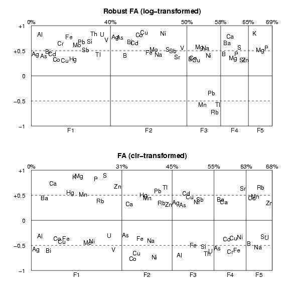
loadplot(res5,titlepl="Robust FA (log-transformed)", crit=0.3)
loadplot(res5logcentr,titlepl="FA (clr-transformed)", crit=0.3)
dev.off()
library(StatDA)
data(moss)
data(kola.background)
X=moss[,"XCOO"]
Y=moss[,"YCOO"]
sel=c("Ag","Al","As","B","Ba","Bi","Ca","Cd","Co","Cr","Cu","Fe","Hg","K","Mg",
"Mn","Mo","Na","Ni","P","Pb","Rb","S","Sb","Si","Sr","Th","Tl","U","V","Zn")
x=log10(moss[,sel])
set.seed(100)
x.mcd=covMcd(x,cor=TRUE)
# robust PFA
res=pfa(x.rsc,factors=5,covmat=x.mcd,scores="regression",rotation="varimax")
# true representation of x and y axis of map for plot
xwid=diff(range(X))/12e4
ywid=diff(range(Y))/12e4
pdf("fig-14-11.pdf",width=2*xwid,height=2*ywid)
par(mfrow=c(2,2),mar=c(1.5,1.5,1.5,1.5))
### NEW MAP:
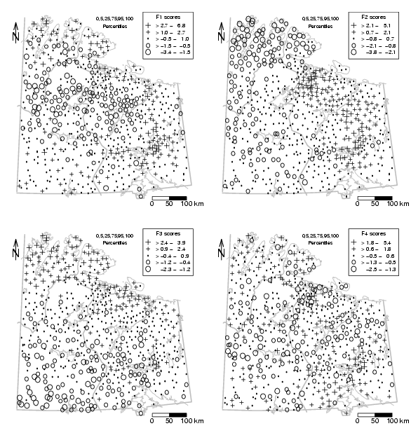
el=res$sco[,1]
# generate plot with background
plot(X,Y,frame.plot=FALSE,xaxt="n",yaxt="n",xlab="",ylab="",type="n")
plotbg(map.col=c("gray","gray","gray","gray"),add.plot=T)
SymbLegend(X,Y,el,type="percentile",qutiles<-c(0,0.05,0.25,0.75,0.95,1),symbtype="EDA",symbmagn=0.8,
leg.position="topright",leg.title="F1 scores",leg.title.cex=0.80,leg.round=1,leg.wid=5,leg.just="right")
# Percentile legend
text(min(X)+diff(range(X))*4/7,max(Y),paste(qutiles*100,collapse=","),cex=0.7)
text(min(X)+diff(range(X))*4/7,max(Y)-diff(range(Y))/25,"Percentiles",cex=0.75)
# scalebar
scalebar(761309,7373050,861309,7363050,shifttext=-0.5,shiftkm=37e3,sizetext=0.8)
# North arrow
Northarrow(362602,7818750,362602,7878750,362602,7838750,Alength=0.15,Aangle=15,Alwd=1.3,Tcex=1.6)
### NEW MAP:
el=res$sco[,2]
# generate plot with background
plot(X,Y,frame.plot=FALSE,xaxt="n",yaxt="n",xlab="",ylab="",type="n")
plotbg(map.col=c("gray","gray","gray","gray"),add.plot=T)
SymbLegend(X,Y,el,type="percentile",qutiles<-c(0,0.05,0.25,0.75,0.95,1),symbtype="EDA",symbmagn=0.8,
leg.position="topright",leg.title="F2 scores",leg.title.cex=0.80,leg.round=1,leg.wid=5,leg.just="right")
# Percentile legend
text(min(X)+diff(range(X))*4/7,max(Y),paste(qutiles*100,collapse=","),cex=0.7)
text(min(X)+diff(range(X))*4/7,max(Y)-diff(range(Y))/25,"Percentiles",cex=0.75)
# scalebar
scalebar(761309,7373050,861309,7363050,shifttext=-0.5,shiftkm=37e3,sizetext=0.8)
# North arrow
Northarrow(362602,7818750,362602,7878750,362602,7838750,Alength=0.15,Aangle=15,Alwd=1.3,Tcex=1.6)
### NEW MAP:
el=res$sco[,3]
# generate plot with background
plot(X,Y,frame.plot=FALSE,xaxt="n",yaxt="n",xlab="",ylab="",type="n")
plotbg(map.col=c("gray","gray","gray","gray"),add.plot=T)
SymbLegend(X,Y,el,type="percentile",qutiles<-c(0,0.05,0.25,0.75,0.95,1),symbtype="EDA",symbmagn=0.8,
leg.position="topright",leg.title="F3 scores",leg.title.cex=0.80,leg.round=1,leg.wid=5,leg.just="right")
# Percentile legend
text(min(X)+diff(range(X))*4/7,max(Y),paste(qutiles*100,collapse=","),cex=0.7)
text(min(X)+diff(range(X))*4/7,max(Y)-diff(range(Y))/25,"Percentiles",cex=0.75)
# scalebar
scalebar(761309,7373050,861309,7363050,shifttext=-0.5,shiftkm=37e3,sizetext=0.8)
# North arrow
Northarrow(362602,7818750,362602,7878750,362602,7838750,Alength=0.15,Aangle=15,Alwd=1.3,Tcex=1.6)
### NEW MAP:
el=res$sco[,4]
# generate plot with background
plot(X,Y,frame.plot=FALSE,xaxt="n",yaxt="n",xlab="",ylab="",type="n")
plotbg(map.col=c("gray","gray","gray","gray"),add.plot=T)
SymbLegend(X,Y,el,type="percentile",qutiles<-c(0,0.05,0.25,0.75,0.95,1),symbtype="EDA",symbmagn=0.8,
leg.position="topright",leg.title="F4 scores",leg.title.cex=0.80,leg.round=1,leg.wid=5,leg.just="right")
# Percentile legend
text(min(X)+diff(range(X))*4/7,max(Y),paste(qutiles*100,collapse=","),cex=0.7)
text(min(X)+diff(range(X))*4/7,max(Y)-diff(range(Y))/25,"Percentiles",cex=0.75)
# scalebar
scalebar(761309,7373050,861309,7363050,shifttext=-0.5,shiftkm=37e3,sizetext=0.8)
# North arrow
Northarrow(362602,7818750,362602,7878750,362602,7838750,Alength=0.15,Aangle=15,Alwd=1.3,Tcex=1.6)
dev.off()
library(StatDA)
data(moss)
data(kola.background)
X=moss[,"XCOO"]
Y=moss[,"YCOO"]
sel=c("Ag","Al","As","B","Ba","Bi","Ca","Cd","Co","Cr","Cu","Fe","Hg","K","Mg",
"Mn","Mo","Na","Ni","P","Pb","Rb","S","Sb","Si","Sr","Th","Tl","U","V","Zn")
x=(moss[,sel])
# Closure problem with log-centring transformation
xgeom=10^apply(log10(x),1,mean)
x2=x/xgeom
x2.obj=log10(x2)
set.seed(200)
st=matrix(runif(31*200),nrow=31)
res5logcentr=pfa(scale(x2.obj),factors=5,scores="Bartlett",rotation="varimax",start=st)
# true representation of x and y axis of map for plot
xwid=diff(range(X))/12e4
ywid=diff(range(Y))/12e4
pdf("fig-14-12.pdf",width=2*xwid,height=2*ywid)
par(mfrow=c(2,2),mar=c(1.5,1.5,1.5,1.5))
### NEW MAP:
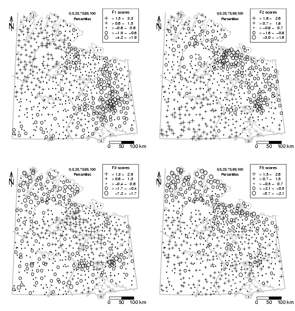
el=res5logcentr$sco[,1]
# generate plot with background
plot(X,Y,frame.plot=FALSE,xaxt="n",yaxt="n",xlab="",ylab="",type="n")
plotbg(map.col=c("gray","gray","gray","gray"),add.plot=T)
SymbLegend(X,Y,el,type="percentile",qutiles<-c(0,0.05,0.25,0.75,0.95,1),symbtype="EDA",symbmagn=0.8,
leg.position="topright",leg.title="F1 scores",leg.title.cex=0.80,leg.round=1,leg.wid=5,leg.just="right")
# Percentile legend
text(min(X)+diff(range(X))*4/7,max(Y),paste(qutiles*100,collapse=","),cex=0.7)
text(min(X)+diff(range(X))*4/7,max(Y)-diff(range(Y))/25,"Percentiles",cex=0.75)
# scalebar
scalebar(761309,7373050,861309,7363050,shifttext=-0.5,shiftkm=37e3,sizetext=0.8)
# North arrow
Northarrow(362602,7818750,362602,7878750,362602,7838750,Alength=0.15,Aangle=15,Alwd=1.3,Tcex=1.6)
### NEW MAP:
el=res5logcentr$sco[,2]
# generate plot with background
plot(X,Y,frame.plot=FALSE,xaxt="n",yaxt="n",xlab="",ylab="",type="n")
plotbg(map.col=c("gray","gray","gray","gray"),add.plot=T)
SymbLegend(X,Y,el,type="percentile",qutiles<-c(0,0.05,0.25,0.75,0.95,1),symbtype="EDA",symbmagn=0.8,
leg.position="topright",leg.title="F2 scores",leg.title.cex=0.80,leg.round=1,leg.wid=5,leg.just="right")
# Percentile legend
text(min(X)+diff(range(X))*4/7,max(Y),paste(qutiles*100,collapse=","),cex=0.7)
text(min(X)+diff(range(X))*4/7,max(Y)-diff(range(Y))/25,"Percentiles",cex=0.75)
# scalebar
scalebar(761309,7373050,861309,7363050,shifttext=-0.5,shiftkm=37e3,sizetext=0.8)
# North arrow
Northarrow(362602,7818750,362602,7878750,362602,7838750,Alength=0.15,Aangle=15,Alwd=1.3,Tcex=1.6)
### NEW MAP:
el=res5logcentr$sco[,3]
# generate plot with background
plot(X,Y,frame.plot=FALSE,xaxt="n",yaxt="n",xlab="",ylab="",type="n")
plotbg(map.col=c("gray","gray","gray","gray"),add.plot=T)
SymbLegend(X,Y,el,type="percentile",qutiles<-c(0,0.05,0.25,0.75,0.95,1),symbtype="EDA",symbmagn=0.8,
leg.position="topright",leg.title="F3 scores",leg.title.cex=0.80,leg.round=1,leg.wid=5,leg.just="right")
# Percentile legend
text(min(X)+diff(range(X))*4/7,max(Y),paste(qutiles*100,collapse=","),cex=0.7)
text(min(X)+diff(range(X))*4/7,max(Y)-diff(range(Y))/25,"Percentiles",cex=0.75)
# scalebar
scalebar(761309,7373050,861309,7363050,shifttext=-0.5,shiftkm=37e3,sizetext=0.8)
# North arrow
Northarrow(362602,7818750,362602,7878750,362602,7838750,Alength=0.15,Aangle=15,Alwd=1.3,Tcex=1.6)
### NEW MAP:
el=res5logcentr$sco[,5]
# generate plot with background
plot(X,Y,frame.plot=FALSE,xaxt="n",yaxt="n",xlab="",ylab="",type="n")
plotbg(map.col=c("gray","gray","gray","gray"),add.plot=T)
SymbLegend(X,Y,el,type="percentile",qutiles<-c(0,0.05,0.25,0.75,0.95,1),symbtype="EDA",symbmagn=0.8,
leg.position="topright",leg.title="F5 scores",leg.title.cex=0.80,leg.round=1,leg.wid=5,leg.just="right")
# Percentile legend
text(min(X)+diff(range(X))*4/7,max(Y),paste(qutiles*100,collapse=","),cex=0.7)
text(min(X)+diff(range(X))*4/7,max(Y)-diff(range(Y))/25,"Percentiles",cex=0.75)
# scalebar
scalebar(761309,7373050,861309,7363050,shifttext=-0.5,shiftkm=37e3,sizetext=0.8)
# North arrow
Northarrow(362602,7818750,362602,7878750,362602,7838750,Alength=0.15,Aangle=15,Alwd=1.3,Tcex=1.6)
dev.off()