library(StatDA)
data(moss)
X=moss[,"XCOO"]
Y=moss[,"YCOO"]
sel=c("Ag","Al","As","B","Ba","Bi","Ca","Cd","Co","Cr","Cu","Fe","Hg","K","Mg",
"Mn","Mo","Na","Ni","P","Pb","Rb","S","Sb","Si","Sr","Th","Tl","U","V","Zn")
x=moss[,sel]
# Closure problem with ilr transformation
ilr <- function(x){
# ilr transformation
x.ilr=matrix(NA,nrow=nrow(x),ncol=ncol(x)-1)
for (i in 1:ncol(x.ilr)){
x.ilr[,i]=sqrt((i)/(i+1))*log(((apply(as.matrix(x[,1:i]), 1, prod))^(1/i))/(x[,i+1]))
}
return(x.ilr)
}
x2=ilr(x)
res2=princomp(x2,cor=TRUE)
x2.mcd=covMcd(x2,cor=T)
res2rob=princomp(x2,covmat=x2.mcd,cor=T)
pdf("fig-14-7.pdf",width=10,height=5)
par(mfcol=c(1,2),mar=c(4,4,4,2))
# construct orthonormal basis: (matrix with 31 rows and 30 columns)
V=matrix(0,nrow=31,ncol=30)
for (i in 1:ncol(V)){
V[1:i,i] <- 1/i
V[i+1,i] <- (-1)
V[,i] <- V[,i]*sqrt(i/(i+1))
}
# log-centred PCA
# Closure problem with log-centring transformation
xgeom=10^apply(log10(x),1,mean)
xlc1=x/xgeom
xlc=log10(xlc1)
reslc=princomp(xlc,cor=TRUE)
# classical result - back-transformed
res2back=res2
res2back$loadings <- V%*%res2$loadings
res2back$scores <- res2$scores%*%t(V)
dimnames(res2back$loadings)[[1]] <- names(x)
res2back$sdev <- apply(res2back$scores,2,sd)
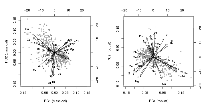
biplot(res2back,xlab="PC1 (classical)",ylab="PC2 (classical)",col=c(gray(0.6),1),
xlabs=rep("+",nrow(x)),cex=0.8)
# robust result - back-transformed
res2robback=res2rob
res2robback$loadings <- V%*%res2rob$loadings
res2robback$scores <- res2rob$scores%*%t(V)
dimnames(res2robback$loadings)[[1]] <- names(x)
res2robback$sdev <- apply(res2robback$scores,2,mad)
biplot(res2robback,xlab="PC1 (robust)",ylab="PC2 (robust)",col=c(gray(0.6),1),
xlabs=rep("+",nrow(x)),cex=0.8)
dev.off()