library(StatDA)
data(moss)
X=moss[,"XCOO"]
Y=moss[,"YCOO"]
sel=c("Ag","Al","As","B","Ba","Bi","Ca","Cd","Co","Cr","Cu","Fe","Hg","K","Mg",
"Mn","Mo","Na","Ni","P","Pb","Rb","S","Sb","Si","Sr","Th","Tl","U","V","Zn")
x=moss[,sel]
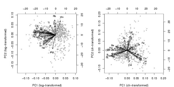
## Closure problem with log-ratio transformation
res.cla=princomp(log10(x),cor=TRUE)
# Closure problem with log-centring transformation
xgeom=10^apply(log10(x),1,mean)
x2=x/xgeom
x2.obj=log10(x2)
res2=princomp(x2.obj,cor=TRUE)
pdf("fig-14-4.pdf",width=10,height=5)
par(mfcol=c(1,2),mar=c(4,4,4,2))
# supress text for Hg and print extra:
dimnames(res.cla$loa)[[1]][13] <- " "
biplot(res.cla,xlab="PC1 (log-transformed)",ylab="PC2 (log-transformed)",col=c(gray(0.6),1),xlabs=rep("+",nrow(x)),cex=0.8)
text(-6,2,"Hg",col=1,cex=0.8)
biplot(res2,xlab="PC1 (clr-transformed)",ylab="PC2 (clr-transformed)",col=c(gray(0.6),1),xlabs=rep("+",nrow(x)),cex=0.8)
dev.off()