library(StatDA)
data(moss)
X=moss[,"XCOO"]
Y=moss[,"YCOO"]
sel=c("Ag","Al","As","B","Ba","Bi","Ca","Cd","Co","Cr","Cu","Fe","Hg","K","Mg",
"Mn","Mo","Na","Ni","P","Pb","Rb","S","Sb","Si","Sr","Th","Tl","U","V","Zn")
x=moss[,sel]
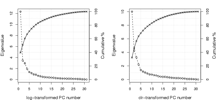
res=eigen(cor(log10(x)))$val
# Closure problem with log-centring transformation
xgeom=10^apply(log10(x),1,mean)
x2=x/xgeom
x2.obj=log10(x2)
res2=eigen(cor(x2.obj))$val
pdf("fig-14-3.pdf",width=10,height=4.5)
par(mfcol=c(1,2),mar=c(4,4,2,5))
plot(res,xlab="log-transformed PC number", ylab="Eigenvalue",
cex.lab=1.2, cex=0.9, pch=1, lwd=1)
abline(v=seq(from=0,by=5,to=ncol(x)),lty=3, col=gray(0.5))
abline(h=seq(from=0,by=0.1,to=1)*res[1],lty=3, col=gray(0.5))
lines(res,lty=2, lwd=1.2)
cumval=cumsum(res)/sum(res)
points(cumval*res[1],pch=4,cex=0.9, lwd=1)
lines(cumval*res[1], lty=1, lwd=1.2)
axis(4, at=seq(0,1,by=0.2)*res[1], labels=seq(0,100,by=20))
mtext("Cumulative %", side=4,line=2.5, cex=1.2)
# log-centred:
plot(res2,xlab="clr-transformed PC number", ylab="Eigenvalue",
cex.lab=1.2, cex=0.9, pch=1, lwd=1)
abline(v=seq(from=0,by=5,to=ncol(x)),lty=3,col=gray(0.5))
abline(h=seq(from=0,by=0.1,to=1)*res2[1],lty=3,col=gray(0.5))
lines(res2,lty=2,lwd=1.2)
cumval=cumsum(res2)/sum(res2)
points(cumval*res2[1],pch=4,cex=0.9,lwd=1)
lines(cumval*res2[1], lty=1,lwd=1.2)
axis(4, at=seq(0,1,by=0.2)*res2[1], labels=seq(0,100,by=20))
mtext("Cumulative %", side=4,line=2.5, cex=1.2)
dev.off()