library(StatDA)
data(moss)
X=moss[,"XCOO"]
Y=moss[,"YCOO"]
el=c("Ag","As","Bi","Cd","Co","Cu","Ni")
x=log10(moss[,el])
data(kola.background)
res <- plotmvoutlier(cbind(X,Y),x,symb=FALSE,map.col=c("grey","grey","grey","grey"),
map.lwd=c(1,1,1,1),plotmap=FALSE,
xlab="",ylab="",frame.plot=FALSE,xaxt="n",yaxt="n")
grp=res$out # Outliers and non-outliers
pdf("fig-13-7.pdf",width=9,height=4.5)
par(mfcol=c(1,2),mar=c(4,4,2,2))
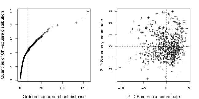
covr <- covMcd(x)
dist <- mahalanobis(x, center = covr$center, cov = covr$cov)
s <- sort(dist, index = TRUE)
q <- (0.5:length(dist))/length(dist)
qchi <- qchisq(q, df = ncol(x))
plot(s$x, qchi, xlab = "Ordered squared robust distance",
ylab = "Quantiles of Chi-square distribution",type="n",cex.lab=1.2)
outl=(s$x>s$x[s$ix==127])
points(s$x[!outl],qchi[!outl],pch=21,cex=0.5)
points(s$x[outl],qchi[outl],pch=3,cex=0.9)
abline(v=s$x[s$ix==127],lty=2)
# Sammon's non-linear mapping
res=sammon(dist(scale(x)))
plot(res$points, xlab="2-D Sammon x-coordinate",ylab="2-D Sammon y-coordinate",cex.lab=1.2,type="n")
points(res$points[grp,],pch=3,cex=0.9)
points(res$points[!grp,],pch=1,cex=0.5)
abline(h=0,lty=2)
abline(v=0,lty=2)
dev.off()
library(StatDA)
# need results from minimum spanning tree function of Bob Garrett:
source("fig-13-8-INPUT.R")
# REMARK: Unfortunately, I did not find an adequate function "mstree" in R
# which gives the same output structure as the Splus function used in
# Bob's programs.
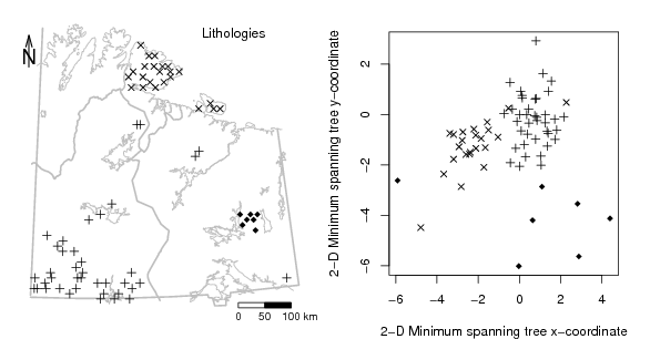
data(chorizon)
data(kola.background)
el=c("Ca","Zn","Mg","Cu","Sr","Na")
x=chorizon[,el]
sel=((chorizon[,"LITO"]==7) |
(chorizon[,"LITO"]==9) | (chorizon[,"LITO"]==82))
grp=chorizon[sel,"LITO"]
grp[grp==7] <- 3
grp[grp==9] <- 4
grp[grp==82] <- 18
x=scale(log10(x[sel,]))
lab=chorizon[sel,"LITO"]
X=chorizon[,"XCOO"]
Y=chorizon[,"YCOO"]
# true representation of x and y axis of map for plot
xwid=diff(range(X))/12e4
ywid=diff(range(Y))/12e4
pdf("fig-13-8.pdf",width=2*xwid,height=1*ywid)
par(mfrow=c(1,2),mar=c(1.5,1.5,1.5,1.5))
# NEW MAP
plot(X,Y,frame.plot=FALSE,xaxt="n",yaxt="n",xlab="",ylab="",type="n")
plotbg(map.col=c("gray","gray","gray","gray"),add.plot=T)
points(chorizon[sel,"XCOO"],chorizon[sel,"YCOO"],col=1,pch=grp)
# scalebar
scalebar(761309,7373050,861309,7363050,shifttext=-0.5,shiftkm=37e3,sizetext=0.8)
# North arrow
Northarrow(362602,7818750,362602,7878750,362602,7838750,Alength=0.15,Aangle=15,Alwd=1.3,Tcex=1.6)
# Legend
text(752000,7880000,"Lithologies",cex=1)
# Results of Bob for minimum spanning trees
res=kola.c.test2.mst
par(mar=c(4,4,2,2))
plot(res$x, res$y, xlab = "2-D Minimum spanning tree x-coordinate",
ylab = "2-D Minimum spanning tree y-coordinate",,main="",pch=grp)
dev.off()