10.5 The Special Case of Closed Number Systems

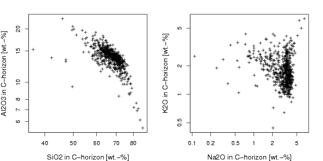
# Fig. 10.7.: Plots showing the closure problem library(StatDA) data(chorizon) x=chorizon[,c("Al2O3","CaO","Fe2O3","K2O","MgO","MnO","Na2O","P2O5","SiO2","TiO2")] pdf("fig-10-7.pdf",width=9,height=4.5) par(mfrow=c(1,2),mar=c(4,4,2,2)) plot(log10(x[,"SiO2"]),log10(x[,"Al2O3"]), xlab="SiO2 in C-horizon [wt.-%]",ylab="Al2O3 in C-horizon [wt.-%]", cex.lab=1.2, pch=3, cex=0.7, xaxt="n", yaxt="n") axis(1,at=log10(a<-sort(c((10^(-50:50))%*%t(c(2,3,4,5,6,7,8,9,10))))),labels=a) axis(2,at=log10(a<-sort(c((10^(-50:50))%*%t(c(1.5,2,3,4,5,6,7,8,10))))),labels=a) plot(log10(x[,"Na2O"]),log10(x[,"K2O"]), xlab="Na2O in C-horizon [wt.-%]",ylab="K2O in C-horizon [wt.-%]", cex.lab=1.2, pch=3, cex=0.7, xaxt="n", yaxt="n") axis(1,at=log10(a<-sort(c((10^(-50:50))%*%t(c(2,5,10))))),labels=a) axis(2,at=log10(a<-sort(c((10^(-50:50))%*%t(c(2,5,10))))),labels=a) dev.off()