9 Comparing Data Using Statistical Tests

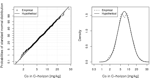
# Fig. 9.1.: QP-plot for Co in C-Horizon library(StatDA) data(chorizon) Co=chorizon[,"Co"] n=length(Co) pdf("fig-9-1.pdf",width=9,height=4.5) par(mfrow=c(1,2),mar=c(4,4,2,2)) qpplot.das(log10(Co),qdist=qnorm,xlab="Co in C-horizon [mg/kg]", lwd=1.5, ylab="Probabilities of standard normal distribution", pch=3,cex=0.7, logx=TRUE, logfinetick=c(2,5,10),logfinelab=c(2,5,10),cex.lab=1.2) legend("topleft",legend=c("Empirical","Hypothetical"),lty=c(NA,1),pch=c(3,NA),cex=0.95,bg="white", lwd=c(NA,1.5)) plot(d <- density(log10(Co)),main="",xlab="Co in C-horizon [mg/kg]",xaxt="n",cex.lab=1.2,lty=2, xlim=c(log10(0.5),log10(50)),ylim=c(0,1.7),lwd=1.5) axis(1,at=log10(a<-sort(c((10^(-50:50))%*%t(c(2,5,10))))),labels=a) lines(d$x,dnorm(d$x,mean(log10(Co)),sd(log10(Co))),lty=1,lwd=1.5) legend("topleft",legend=c("Empirical","Hypothetical"),lty=c(2,1),lwd=c(1.5,1.5),cex=0.95) dev.off()

# Statistical testing: R scipts

# Distribution tests:
library(mvoutlier)
data(chorizon)
Co=chorizon[,"Co"]


ks.test(log(Co),"pnorm",mean(log(Co)),sd(log(Co)))

One-sample Kolmogorov-Smirnov test

data: log(Co)
D = 0.0296, p-value = 0.6613
alternative hypothesis: two.sided

shapiro.test(log(Co))

Shapiro-Wilk normality test

data: log(Co)
W = 0.9983, p-value = 0.8399


As=chorizon[,"As"]
ks.test(log(As),"pnorm",mean(log(As)),sd(log(As)))
shapiro.test(log(As))



# t-Test
Cu=chorizon[,"Cu"]
exp(mean(log(Cu)))
[1] 16.59534
> t.test(log(chorizon[,"Cu"]),mu=log(18))

coun=chorizon[,"COUN"]
t.test(log(chorizon[coun=="FIN","Cu"]),mu=log(18))
t.test(log(chorizon[coun=="NOR","Cu"]),mu=log(18))
t.test(log(chorizon[coun=="RUS","Cu"]),mu=log(18))

# Wilcoxon Signed rank test
wilcox.test(log(chorizon[,"Cu"]),mu=log(18))

wilcox.test(log(chorizon[coun=="FIN","Cu"]),mu=log(18))
wilcox.test(log(chorizon[coun=="NOR","Cu"]),mu=log(18))
wilcox.test(log(chorizon[coun=="RUS","Cu"]),mu=log(18))

t.test(log(chorizon[,"As"]),mu=log(18))
wilcox.test(log(chorizon[,"As"]),mu=log(18))

# 2-sample t-Test
coun=chorizon[,"COUN"]
Cu1.l=log(chorizon[coun=="FIN","Cu"])
ks.test(Cu1.l,"pnorm",mean(Cu1.l),sd(Cu1.l))
shapiro.test(Cu1.l)

boxplot(log(chorizon[coun=="FIN","Cu"]),log(chorizon[coun=="NOR","Cu"]),log(chorizon[coun=="RUS","Cu"]),notch=T)

Cu12.l=log(chorizon[coun!="RUS","Cu"])
shapiro.test(log(chorizon[coun!="RUS","Cu"]))
ks.test(Cu12.l,"pnorm",mean(Cu12.l),sd(Cu12.l))

t.test(log(chorizon[coun!="RUS","Cu"]),log(chorizon[coun=="RUS","Cu"]))
t.test(log(chorizon[coun!="RUS","Cu"]),log(chorizon[coun=="RUS","Cu"]),var.equal=T)
boxplot(log(chorizon[coun!="RUS","Cu"]),log(chorizon[coun=="RUS","Cu"]),notch=T)
var.test(log(chorizon[coun!="RUS","Cu"]),log(chorizon[coun=="RUS","Cu"]))
wilcox.test(log(chorizon[coun!="RUS","Cu"]),log(chorizon[coun=="RUS","Cu"]))

# paired t test
# COmpare B- C-horizon
# same locations:
library(mvoutlier)
data(chorizon)
data(bhorizon)
data(moss)
data(humus)
# WIch samples on the same site?
c.ind=NULL
b.ind=NULL
m.ind=NULL
h.ind=NULL
c.id=chorizon[,1]
b.id=bhorizon[,1]
m.id=moss[,1]
h.id=humus[,1]
for (i in 1:1000){
if (sum(c.id==i)+sum(b.id==i)+sum(m.id==i)+sum(h.id==i)==4){
c.ind=c(c.ind,which(c.id==i))
b.ind=c(b.ind,which(b.id==i))
m.ind=c(m.ind,which(m.id==i))
h.ind=c(h.ind,which(h.id==i))
}
}

# Cu-Daten
c.Cul=log(chorizon[c.ind,"Cu"])
b.Cul=log(bhorizon[b.ind,"Cu"])

plot(c.Cul,b.Cul)
t.test(c.Cul,b.Cul,paired=TRUE)
boxplot(c.Cul,b.Cul,notch=T)
t.test(c.Cul,b.Cul,paired=TRUE)
# Normal distribution?
shapiro.test(c.Cul)
shapiro.test(b.Cul)

# Wilcoxon signed rank test
wilcox.test(c.Cul,b.Cul,paired=TRUE)


# Test of variances
var.test(log(chorizon[coun!="RUS","Cu"]),log(chorizon[coun=="RUS","Cu"]))
ansari.test(log(chorizon[coun!="RUS","Cu"]),log(chorizon[coun=="RUS","Cu"]))


# Anova
boxplot(log(chorizon[,"Cu"])~chorizon[,"COUN"])
anova(lm(log(chorizon[,"Cu"])~chorizon[,"COUN"]))

kruskal.test(log(chorizon[,"Cu"]),chorizon[,"COUN"])

bartlett.test(log(chorizon[,"Cu"])~chorizon[,"COUN"])

fligner.test(log(chorizon[,"Cu"])~chorizon[,"COUN"])

library(car)
levene.test(log(chorizon[,"Cu"]),chorizon[,"COUN"])


# k dependent groups
# Cu-data
c.Cul=log(chorizon[c.ind,"Cu"])
b.Cul=log(bhorizon[b.ind,"Cu"])
m.Cul=log(moss[m.ind,"Cu"])
h.Cul=log(humus[h.ind,"Cu"])

boxplot(c.Cul,b.Cul,m.Cul,h.Cul)

# blocked ANOVA:
n=length(c.Cul)
Cuall=c(c.Cul,b.Cul,m.Cul,h.Cul)
N=rep(1:n,4)
datall=data.frame(block=gl(4,n),N=factor(N),Cuall=Cuall)
datall.aov=aov(Cuall~block+N, datall)
summary(datall.aov)
Df Sum Sq Mean Sq F value Pr(>F)
block 3 102.14 34.05 77.6871 < 2.2e-16 ***
N 580 734.93 1.27 2.8913 < 2.2e-16 ***
Residuals 1740 762.55 0.44
---
Signif. codes: 0 `***' 0.001 `**' 0.01 `*' 0.05 `.' 0.1 ` ' 1


friedman.test(cbind(c.Cul,b.Cul,m.Cul,h.Cul))
Friedman rank sum test

data: cbind(c.Cul, b.Cul, m.Cul, h.Cul)
Friedman chi-squared = 293.3056, df = 3, p-value < 2.2e-16




B1=c(36,23,31,47,32)
B2=c(31,14,25,39,27)
B3=c(29,20,22,32,31)
B4=c(14,8,16,18,12)
B=c(B1,B2,B3,B4)
N=rep(1:5,4)
datall=data.frame(block=gl(4,5),N=factor(N),B=B)
datall.aov=aov(B~block+N, datall)
summary(datall.aov)

boxplot(B1,B2,B3,B4)
friedman.test(cbind(B1,B2,B3,B4))




var="Cu"
c.Cul=log(chorizon[c.ind,var])
b.Cul=log(bhorizon[b.ind,var])
m.Cul=log(moss[m.ind,var])
h.Cul=log(humus[h.ind,var])

boxplot(c.Cul,b.Cul,m.Cul,h.Cul,notch=T)

# blocked ANOVA:
n=length(c.Cul)
Cuall=c(c.Cul,b.Cul,m.Cul,h.Cul)
N=rep(1:n,4)
datall=data.frame(block=gl(4,n),N=factor(N),Cuall=Cuall)
datall.aov=aov(Cuall~block+N, datall)
summary(datall.aov)


friedman.test(cbind(c.Cul,b.Cul,m.Cul,h.Cul))