library(StatDA)
# need also this package:
library(sgeostat)
# need data:
data(timetrend)
pH=timetrend[,"pH"]
EC=timetrend[,"EC"]
ca=timetrend[,"Catch"]
x=timetrend[,"YY"]+(timetrend[,"MM"]-1)/12+(timetrend[,"DD"]-1)/365
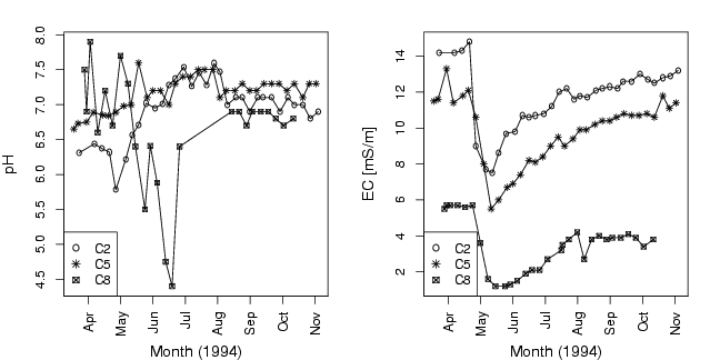
pdf("fig-8-10.pdf",width=9,height=4.5)
par(mfrow=c(1,2),mar=c(4,4,2,2))
plot(x,pH,xlab="Month (1994)", ylab="pH", xaxt="n", type="n",cex.lab=1.2)
axis(1,at=seq(1994,by=1/12,length=12),
labels=c("Jan","Feb","Mar","Apr","May","Jun","Jul","Aug","Sep","Oct","Nov","Dec"),las=3)
points(x[ca==2],pH[ca==2],type="p",pch=1,lty=1,cex=0.8)
points(x[ca==2],pH[ca==2],type="l",pch=1,lty=1,cex=0.8)
points(x[ca==5],pH[ca==5],type="p",pch=8,lty=1,cex=0.8)
points(x[ca==5],pH[ca==5],type="l",pch=8,lty=1,cex=0.8)
points(x[ca==8][!is.na(pH[ca==8])],pH[ca==8][!is.na(pH[ca==8])],type="p",pch=7,lty=1,cex=0.8)
points(x[ca==8][!is.na(pH[ca==8])],pH[ca==8][!is.na(pH[ca==8])],type="l",pch=7,lty=1,cex=0.8)
legend("bottomleft",legend=c("C2","C5","C8"),pch=c(1,8,7))
plot(x,EC,xlab="Month (1994)", ylab="EC [mS/m]", xaxt="n", type="n",cex.lab=1.2)
axis(1,at=seq(1994,by=1/12,length=12),
labels=c("Jan","Feb","Mar","Apr","May","Jun","Jul","Aug","Sep","Oct","Nov","Dec"),las=3)
points(x[ca==2],EC[ca==2],type="p",pch=1,lty=1,cex=0.8)
points(x[ca==2],EC[ca==2],type="l",pch=1,lty=1,cex=0.8)
points(x[ca==5],EC[ca==5],type="p",pch=8,lty=1,cex=0.8)
points(x[ca==5],EC[ca==5],type="l",pch=8,lty=1,cex=0.8)
points(x[ca==8],EC[ca==8],type="p",pch=7,lty=1,cex=0.8)
points(x[ca==8],EC[ca==8],type="l",pch=7,lty=1,cex=0.8)
legend("bottomleft",legend=c("C2","C5","C8"),pch=c(1,8,7))
dev.off()
library(StatDA)
data(ohorizon)
data(chorizon)
data(moss)
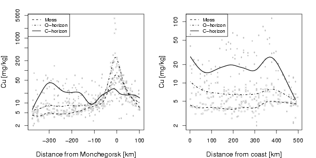
pdf("fig-8-11.pdf",width=9,height=4.5)
par(mfrow=c(1,2),mar=c(4,4,2,2))
X=ohorizon[,"XCOO"]
Y=ohorizon[,"YCOO"]
x1h=(X[Y<7600000 & Y>7500000]-753970)/1000
y1h=log10(ohorizon[Y<7600000 & Y>7500000,"Cu"])
X=moss[,"XCOO"]
Y=moss[,"YCOO"]
x1m=(X[Y<7600000 & Y>7500000]-753970)/1000
y1m=log10(moss[Y<7600000 & Y>7500000,"Cu"])
X=chorizon[,"XCOO"]
Y=chorizon[,"YCOO"]
x1c=(X[Y<7600000 & Y>7500000]-753970)/1000
y1c=log10(chorizon[Y<7600000 & Y>7500000,"Cu"])
plot(x1h,y1h,xlab="Distance from Monchegorsk [km]",ylab="Cu [mg/kg]",pch=4,cex=0.5,
ylim=c(min(y1h,y1m,y1c),max(y1h,y1m,y1c)),yaxt="n",col="gray",cex.lab=1.2)
axis(2,at=log10(a<-sort(c((10^(-50:50))%*%t(c(2,5,10))))),labels=a)
lines(smooth.spline(x1h,y1h,spar=0.7),col=1,lwd=1.4,lty=4)
points(x1m,y1m,pch=22,cex=0.5,col="gray")
lines(smooth.spline(x1m,y1m,spar=0.7),col=1,lty=2,lwd=1.4)
points(x1c,y1c,pch=16,cex=0.3,col="gray")
lines(smooth.spline(x1c,y1c,spar=0.7),col=1,lty=1,lwd=1.4)
legend("topleft",legend=c("Moss","O-horizon","C-horizon"),lty=c(2,4,1),
cex=0.8,lwd=c(1.4,1.4,1.4))
X=ohorizon[,"XCOO"]
Y=ohorizon[,"YCOO"]
x1h=abs((Y[X<460000]-max(Y)+2000)/1000)
y1h=log10(ohorizon[X<460000,"Cu"])
X=moss[,"XCOO"]
Y=moss[,"YCOO"]
x1m=abs((Y[X<460000]-max(Y)+2000)/1000)
y1m=log10(moss[X<460000,"Cu"])
X=chorizon[,"XCOO"]
Y=chorizon[,"YCOO"]
x1c=abs((Y[X<460000]-max(Y)+2000)/1000)
y1c=log10(chorizon[X<460000,"Cu"])
plot(x1h,y1h,xlab="Distance from coast [km]",ylab="Cu [mg/kg]",pch=4,cex=0.5,
ylim=c(min(y1h,y1m,y1c),max(y1h,y1m,y1c)),yaxt="n",col="gray",cex.lab=1.2)
axis(2,at=log10(a<-sort(c((10^(-50:50))%*%t(c(2,5,10))))),labels=a)
lines(smooth.spline(x1h,y1h,spar=0.7),col=1,lwd=1.4,lty=4)
points(x1m,y1m,pch=22,cex=0.5,col="gray")
lines(smooth.spline(x1m,y1m,spar=0.7),col=1,lty=2,lwd=1.4)
points(x1c,y1c,pch=16,cex=0.3,col="gray")
lines(smooth.spline(x1c,y1c,spar=0.7),col=1,lty=1,lwd=1.4)
legend("topleft",legend=c("Moss","O-horizon","C-horizon"),lty=c(2,4,1),
cex=0.8,lwd=c(1.4,1.4,1.4))
dev.off()