8.3 Comparing the Spatial Data Structure

# Fig. 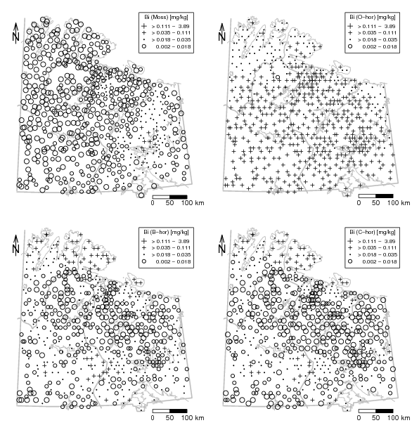8.4.: Bi in 4 layers, percentiles corresponding to all 4 layers jointly library(StatDA) data(chorizon) data(bhorizon) data(moss) data(ohorizon) data(kola.background) X=chorizon[,"XCOO"] Y=chorizon[,"YCOO"] # true representation of x and y axis of map for plot xwid=diff(range(X))/12e4 ywid=diff(range(Y))/12e4 pdf("fig-8-4.pdf",width=2*xwid,height=2*ywid) par(mfrow=c(2,2),mar=c(1.5,1.5,1.5,1.5)) el.M=moss[,"Bi"] el.O=ohorizon[,"Bi"] el.B=bhorizon[,"Bi"] el.C=chorizon[,"Bi"] ### NEW MAP: el=moss[,"Bi"] X=moss[,"XCOO"] Y=moss[,"YCOO"] # generate plot with background plot(X,Y,frame.plot=FALSE,xaxt="n",yaxt="n",xlab="",ylab="",type="n") plotbg(map.col=c("gray","gray","gray","gray"),add.plot=T) qutiles <- c(0,0.05,0.25,0.75,0.98,1) SymbLegend(X,Y,el,type="percentile",qutiles=qutiles, q=quantile(c(el.M,el.O,el.B,el.C), qutiles=qutiles), symbtype="EDA",symbmagn=0.8, leg.position="topright",leg.title="Bi (Moss) [mg/kg]", leg.title.cex=0.8,leg.round=3,leg.wid=5,leg.just="right") # scalebar scalebar(761309,7373050,861309,7363050,shifttext=-0.5,shiftkm=37e3,sizetext=0.8) # North arrow Northarrow(362602,7818750,362602,7878750,362602,7838750,Alength=0.15,Aangle=15,Alwd=1.3,Tcex=1.6) ### NEW MAP: el=ohorizon[,"Bi"] X=ohorizon[,"XCOO"] Y=ohorizon[,"YCOO"] # generate plot with background plot(X,Y,frame.plot=FALSE,xaxt="n",yaxt="n",xlab="",ylab="",type="n") plotbg(map.col=c("gray","gray","gray","gray"),add.plot=T) SymbLegend(X,Y,el,type="percentile",qutiles=qutiles, q=quantile(c(el.M,el.O,el.B,el.C), qutiles=qutiles), symbtype="EDA",symbmagn=0.8, leg.position="topright",leg.title="Bi (O-hor) [mg/kg]", leg.title.cex=0.8,leg.round=3,leg.wid=5,leg.just="right") # scalebar scalebar(761309,7373050,861309,7363050,shifttext=-0.5,shiftkm=37e3,sizetext=0.8) # North arrow Northarrow(362602,7818750,362602,7878750,362602,7838750,Alength=0.15,Aangle=15,Alwd=1.3,Tcex=1.6) ### NEW MAP: el=bhorizon[,"Bi"] X=bhorizon[,"XCOO"] Y=bhorizon[,"YCOO"] # generate plot with background plot(X,Y,frame.plot=FALSE,xaxt="n",yaxt="n",xlab="",ylab="",type="n") plotbg(map.col=c("gray","gray","gray","gray"),add.plot=T) SymbLegend(X,Y,el,type="percentile",qutiles=qutiles, q=quantile(c(el.M,el.O,el.B,el.C), qutiles=qutiles), symbtype="EDA",symbmagn=0.8, leg.position="topright",leg.title="Bi (B-hor) [mg/kg]", leg.title.cex=0.8,leg.round=3,leg.wid=5,leg.just="right") # scalebar scalebar(761309,7373050,861309,7363050,shifttext=-0.5,shiftkm=37e3,sizetext=0.8) # North arrow Northarrow(362602,7818750,362602,7878750,362602,7838750,Alength=0.15,Aangle=15,Alwd=1.3,Tcex=1.6) ### NEW MAP: el=chorizon[,"Bi"] X=chorizon[,"XCOO"] Y=chorizon[,"YCOO"] # generate plot with background plot(X,Y,frame.plot=FALSE,xaxt="n",yaxt="n",xlab="",ylab="",type="n") plotbg(map.col=c("gray","gray","gray","gray"),add.plot=T) SymbLegend(X,Y,el,type="percentile",qutiles=qutiles, q=quantile(c(el.M,el.O,el.B,el.C), qutiles=qutiles), symbtype="EDA",symbmagn=0.8, leg.position="topright",leg.title="Bi (C-hor) [mg/kg]", leg.title.cex=0.8,leg.round=3,leg.wid=5,leg.just="right") # scalebar scalebar(761309,7373050,861309,7363050,shifttext=-0.5,shiftkm=37e3,sizetext=0.8) # North arrow Northarrow(362602,7818750,362602,7878750,362602,7838750,Alength=0.15,Aangle=15,Alwd=1.3,Tcex=1.6) dev.off()

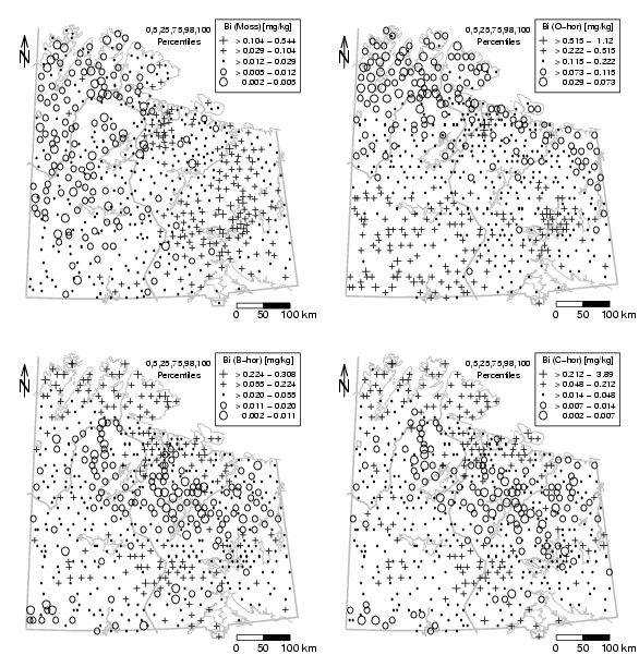
# Fig. 8.5.: Bi in 4 layers, same scale library(StatDA) data(chorizon) data(bhorizon) data(moss) data(ohorizon) data(kola.background) X=chorizon[,"XCOO"] Y=chorizon[,"YCOO"] # true representation of x and y axis of map for plot xwid=diff(range(X))/12e4 ywid=diff(range(Y))/12e4 pdf("fig-8-5.pdf",width=2*xwid,height=2*ywid) par(mfrow=c(2,2),mar=c(1.5,1.5,1.5,1.5)) ### NEW MAP: el=moss[,"Bi"] X=moss[,"XCOO"] Y=moss[,"YCOO"] # generate plot with background plot(X,Y,frame.plot=FALSE,xaxt="n",yaxt="n",xlab="",ylab="",type="n") plotbg(map.col=c("gray","gray","gray","gray"),add.plot=T) SymbLegend(X,Y,el,type="percentile",qutiles<-c(0,0.05,0.25,0.75,0.98,1),symbtype="EDA",symbmagn=0.8, leg.position="topright",leg.title="Bi (Moss) [mg/kg]",leg.title.cex=0.8,leg.round=3,leg.wid=5,leg.just="right") # Text text(min(X)+diff(range(X))*4/7,max(Y),paste(qutiles*100,collapse=","),cex=0.8) text(min(X)+diff(range(X))*4/7,max(Y)-diff(range(Y))/25,"Percentiles",cex=0.8) # scalebar scalebar(761309,7373050,861309,7363050,shifttext=-0.5,shiftkm=37e3,sizetext=0.8) # North arrow Northarrow(362602,7818750,362602,7878750,362602,7838750,Alength=0.15,Aangle=15,Alwd=1.3,Tcex=1.6) ### NEW MAP: el=ohorizon[,"Bi"] X=ohorizon[,"XCOO"] Y=ohorizon[,"YCOO"] # generate plot with background plot(X,Y,frame.plot=FALSE,xaxt="n",yaxt="n",xlab="",ylab="",type="n") plotbg(map.col=c("gray","gray","gray","gray"),add.plot=T) SymbLegend(X,Y,el,type="percentile",qutiles<-c(0,0.05,0.25,0.75,0.98,1),symbtype="EDA",symbmagn=0.8, leg.position="topright",leg.title="Bi (O-hor) [mg/kg]",leg.title.cex=0.8,leg.round=3,leg.wid=5,leg.just="right") # Text text(min(X)+diff(range(X))*4/7,max(Y),paste(qutiles*100,collapse=","),cex=0.8) text(min(X)+diff(range(X))*4/7,max(Y)-diff(range(Y))/25,"Percentiles",cex=0.8) # scalebar scalebar(761309,7373050,861309,7363050,shifttext=-0.5,shiftkm=37e3,sizetext=0.8) # North arrow Northarrow(362602,7818750,362602,7878750,362602,7838750,Alength=0.15,Aangle=15,Alwd=1.3,Tcex=1.6) ### NEW MAP: el=bhorizon[,"Bi"] X=bhorizon[,"XCOO"] Y=bhorizon[,"YCOO"] # generate plot with background plot(X,Y,frame.plot=FALSE,xaxt="n",yaxt="n",xlab="",ylab="",type="n") plotbg(map.col=c("gray","gray","gray","gray"),add.plot=T) SymbLegend(X,Y,el,type="percentile",qutiles<-c(0,0.05,0.25,0.75,0.98,1),symbtype="EDA",symbmagn=0.8, leg.position="topright",leg.title="Bi (B-hor) [mg/kg]",leg.title.cex=0.8,leg.round=3,leg.wid=5,leg.just="right") # Text text(min(X)+diff(range(X))*4/7,max(Y),paste(qutiles*100,collapse=","),cex=0.8) text(min(X)+diff(range(X))*4/7,max(Y)-diff(range(Y))/25,"Percentiles",cex=0.8) # scalebar scalebar(761309,7373050,861309,7363050,shifttext=-0.5,shiftkm=37e3,sizetext=0.8) # North arrow Northarrow(362602,7818750,362602,7878750,362602,7838750,Alength=0.15,Aangle=15,Alwd=1.3,Tcex=1.6) ### NEW MAP: el=chorizon[,"Bi"] X=chorizon[,"XCOO"] Y=chorizon[,"YCOO"] # generate plot with background plot(X,Y,frame.plot=FALSE,xaxt="n",yaxt="n",xlab="",ylab="",type="n") plotbg(map.col=c("gray","gray","gray","gray"),add.plot=T) SymbLegend(X,Y,el,type="percentile",qutiles<-c(0,0.05,0.25,0.75,0.98,1),symbtype="EDA",symbmagn=0.8, leg.position="topright",leg.title="Bi (C-hor) [mg/kg]",leg.title.cex=0.8,leg.round=3,leg.wid=5,leg.just="right") # Text text(min(X)+diff(range(X))*4/7,max(Y),paste(qutiles*100,collapse=","),cex=0.8) text(min(X)+diff(range(X))*4/7,max(Y)-diff(range(Y))/25,"Percentiles",cex=0.8) # scalebar scalebar(761309,7373050,861309,7363050,shifttext=-0.5,shiftkm=37e3,sizetext=0.8) # North arrow Northarrow(362602,7818750,362602,7878750,362602,7838750,Alength=0.15,Aangle=15,Alwd=1.3,Tcex=1.6) dev.off()