library(StatDA)
data(ohorizon)
X=ohorizon[,"XCOO"]
Y=ohorizon[,"YCOO"]
pdf("fig-7-5.pdf",width=8,height=8)
par(mfrow=c(2,2),mar=c(4,4,2,2))
#####################################################
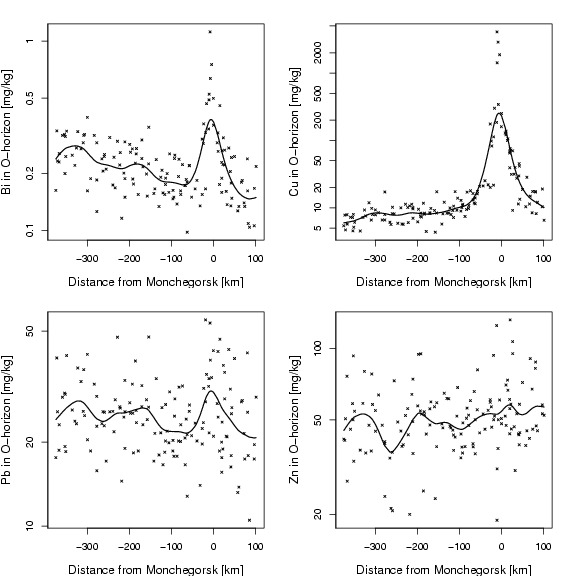
x1h=(X[Y<7600000 & Y>7500000]-753970)/1000
y1h=log10(ohorizon[Y<7600000 & Y>7500000,"Bi"])
plot(x1h,y1h,xlab="Distance from Monchegorsk [km]",ylab="Bi in O-horizon [mg/kg]",pch=4,cex=0.5,
yaxt="n",col=1,cex.lab=1.2)
axis(2,at=log10(a<-sort(c((10^(-50:50))%*%t(c(2,5,10))))),labels=a)
lines(smooth.spline(x1h,y1h,spar=0.7),col=1,lwd=1.4,lty=1)
#####################################################
x1h=(X[Y<7600000 & Y>7500000]-753970)/1000
y1h=log10(ohorizon[Y<7600000 & Y>7500000,"Cu"])
plot(x1h,y1h,xlab="Distance from Monchegorsk [km]",ylab="Cu in O-horizon [mg/kg]",pch=4,cex=0.5,
yaxt="n",col=1,cex.lab=1.2)
axis(2,at=log10(a<-sort(c((10^(-50:50))%*%t(c(2,5,10))))),labels=a)
lines(smooth.spline(x1h,y1h,spar=0.7),col=1,lwd=1.4,lty=1)
#####################################################
x1h=(X[Y<7600000 & Y>7500000]-753970)/1000
y1h=log10(ohorizon[Y<7600000 & Y>7500000,"Pb"])
plot(x1h,y1h,xlab="Distance from Monchegorsk [km]",ylab="Pb in O-horizon [mg/kg]",pch=4,cex=0.5,
yaxt="n",col=1,cex.lab=1.2)
axis(2,at=log10(a<-sort(c((10^(-50:50))%*%t(c(2,5,10))))),labels=a)
lines(smooth.spline(x1h,y1h,spar=0.7),col=1,lwd=1.4,lty=1)
#####################################################
x1h=(X[Y<7600000 & Y>7500000]-753970)/1000
y1h=log10(ohorizon[Y<7600000 & Y>7500000,"Zn"])
plot(x1h,y1h,xlab="Distance from Monchegorsk [km]",ylab="Zn in O-horizon [mg/kg]",pch=4,cex=0.5,
yaxt="n",col=1,cex.lab=1.2)
axis(2,at=log10(a<-sort(c((10^(-50:50))%*%t(c(2,5,10))))),labels=a)
lines(smooth.spline(x1h,y1h,spar=0.7),col=1,lwd=1.4,lty=1)
dev.off()