library(StatDA)
# need data:
data(timetrend)
ca=timetrend[,"Catch"]
#x=timetrend[,"YY"]+(timetrend[,"MM"]-1)/12+(timetrend[,"DD"]-1)/365
x=timetrend[ca==2,"YY"]+(timetrend[ca==2,"MM"]-1)/12+(timetrend[ca==2,"DD"]-1)/365
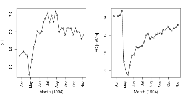
pH=timetrend[ca==2,"pH"]
EC=timetrend[ca==2,"EC"]
pdf("fig-6-5.pdf",width=9,height=4.5)
par(mfrow=c(1,2),mar=c(4,4,2,2))
plot(x,pH,xlab="Month (1994)", ylab="pH", xaxt="n", type="n",cex.lab=1.2)
axis(1,at=seq(1994,by=1/12,length=12),
labels=c("Jan","Feb","Mar","Apr","May","Jun","Jul","Aug","Sep","Oct","Nov","Dec"),las=3)
points(x[ca==2],pH[ca==2],type="p",pch=1,lty=1,cex=0.8)
points(x[ca==2],pH[ca==2],type="l",pch=1,lty=1,cex=0.8)
#points(x[ca==5],pH[ca==5],type="p",pch=8,lty=1,cex=0.8)
#points(x[ca==5],pH[ca==5],type="l",pch=8,lty=1,cex=0.8)
#points(x[ca==8][!is.na(pH[ca==8])],pH[ca==8][!is.na(pH[ca==8])],type="p",pch=7,lty=1,cex=0.8)
#points(x[ca==8][!is.na(pH[ca==8])],pH[ca==8][!is.na(pH[ca==8])],type="l",pch=7,lty=1,cex=0.8)
#legend("bottomleft",legend=c("C2","C5","C8"),pch=c(1,8,7))
plot(x,EC,xlab="Month (1994)", ylab="EC [mS/m]", xaxt="n", type="n",cex.lab=1.2)
axis(1,at=seq(1994,by=1/12,length=12),
labels=c("Jan","Feb","Mar","Apr","May","Jun","Jul","Aug","Sep","Oct","Nov","Dec"),las=3)
points(x,EC,type="p",pch=1,lty=1,cex=0.8)
points(x,EC,type="l",pch=1,lty=1,cex=0.8)
dev.off()