library(StatDA)
pdf("fig-6-2.pdf",width=9,height=4.5)
par(mfrow=c(1,2),mar=c(4,4,2,2))
data(chorizon)
La=chorizon[,"La"]
LaINAA=chorizon[,"La_INAA"]
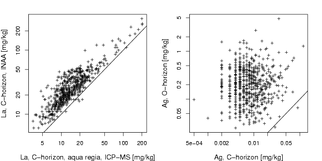
plot(log10(La),log10(LaINAA),xlab="La, C-horizon, aqua regia, ICP-MS [mg/kg]",
ylab="La, C-horizon, INAA [mg/kg]", pch=3, cex=0.7, cex.lab=1.2,xaxt="n",
yaxt="n")
axis(1,at=log10(a<-sort(c((10^(-50:50))%*%t(c(2,5,10))))),labels=a)
axis(2,at=log10(a<-sort(c((10^(-50:50))%*%t(c(2,5,10))))),labels=a)
abline(a=0,b=1)
data(ohorizon)
# only samples from same locations in both layers:
c.ind=NULL
h.ind=NULL
c.id=chorizon[,1]
h.id=ohorizon[,1]
for (i in 1:1000){
if (sum(c.id==i)+sum(h.id==i)==2){
c.ind=c(c.ind,which(c.id==i))
h.ind=c(h.ind,which(h.id==i))
}
}
AgO=ohorizon[h.ind,"Ag"]
AgC=chorizon[c.ind,"Ag"]
plot(log10(AgC),log10(AgO),xlab="Ag, C-horizon [mg/kg]",
ylab="Ag, O-horizon [mg/kg]", pch=3, cex=0.7, cex.lab=1.2,xaxt="n",
yaxt="n")
axis(1,at=log10(a<-sort(c((10^(-50:50))%*%t(c(2,5,10))))),labels=a)
axis(2,at=log10(a<-sort(c((10^(-50:50))%*%t(c(2,5,10))))),labels=a)
abline(a=0,b=1)
dev.off()