library(StatDA)
data(chorizon)
Ba=chorizon[,"Ba"]
pdf("fig-3-5.pdf",width=9,height=7)
par(mfrow=c(2,2),mar=c(4,4,3,3))
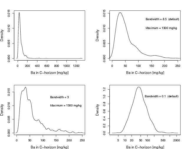
plot(density(Ba),main="",xlab="Ba in C-horizon [mg/kg]",cex.lab=1.2)
plot(d <- density(Ba),main="",xlab="Ba in C-horizon [mg/kg]",xlim=c(0,250),cex.lab=1.2)
text(120,0.013,paste("Bandwidth =",round(d$bw,1)," (default)"),pos=4)
text(120,0.01,paste("Maximum =",max(Ba),"mg/kg"),pos=4)
plot(d <- density(Ba,bw=3),main="",xlab="Ba in C-horizon [mg/kg]",xlim=c(0,250),cex.lab=1.2)
text(120,0.013,paste("Bandwidth =",round(d$bw,1)),pos=4)
text(120,0.01,paste("Maximum =",max(Ba),"mg/kg"),pos=4)
plot(d <- density(log10(Ba)),main="",xlab="Ba in C-horizon [mg/kg]",xaxt="n",cex.lab=1.2)
axis(1,at=log10(a<-sort(c((10^(-50:50))%*%t(c(2,5,10))))),labels=a)
text(1.8,1,paste("Bandwidth =",round(d$bw,1)," (default)"),pos=4)
dev.off()