library(StatDA)
data(chorizon)
Ba=chorizon[,"Ba"]
pdf("fig-3-3.pdf",width=9,height=7)
par(mfrow=c(2,2),mar=c(4,4,3,3))
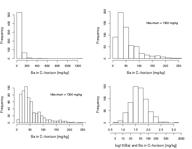
hist(Ba,main="",xlab="Ba in C-horizon [mg/kg]",ylab="Frequency",cex.lab=1.2)
hist(Ba,main="",xlab="Ba in C-horizon [mg/kg]",ylab="Frequency",xlim=c(0,250),breaks=60,cex.lab=1.2)
text(120,150,paste("Maximum =",max(Ba),"mg/kg"),pos=4)
par(mar=c(7,4,3,3))
hist(Ba,main="",xlab="Ba in C-horizon [mg/kg]",ylab="Frequency",xlim=c(0,250),breaks=100,cex.lab=1.2)
text(120,80,paste("Maximum =",max(Ba),"mg/kg"),pos=4)
hist(log10(Ba),main="",xlab="",ylab="Frequency",cex.lab=1.2)
axis(1,at=log10(a<-sort(c((10^(-50:50))%*%t(c(2,5,10))))),labels=a,line=2.5)
mtext("log10(Ba) and Ba in C-horizon [mg/kg]",line=5.5,cex=1,side=1)
dev.off()
library(StatDA)
data(chorizon)
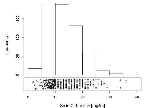
Sc=chorizon[,"Sc_INAA"]
# Function for histogram plus one-dimensional scatter plot:
hist1 <- function(x,xlab,ylab) {
par(oma=c(4,3,0,0), mar=c(0,0,0,0))
layout(matrix(c(1,2),2,1), c(9,9), c(6,1), TRUE)
h <- hist(x, freq=TRUE, axes=FALSE, xlab="", ylab="", main="")
axis(2)
plot(0, 0, type="n", ylim=c(-0.1,1.1), xlim=c(h$breaks[1],h$breaks[length(h$breaks)]),
axes=FALSE, xlab="", ylab="")
mtext(ylab,side=2,line=1,outer=TRUE, las=3,cex=1.2)
box()
set.seed(1)
points(x, runif(length(x)),pch=3,cex=0.5)
axis(1)
mtext(xlab,side=1,line=3,outer=TRUE, las=1,cex=1.2)
}
pdf("fig-3-4.pdf",width=7,height=5)
par(mar=c(2,2,1,1))
hist1(Sc,xlab="Sc in C-horizon [mg/kg]",ylab="Frequency")
dev.off()